Chapter 2: Tests for Two Continuous Population Mean

This chapter introduces statistical tests designed to compare two samples which is a fundamental task in data analysis across many disciplines. Whether you’re comparing average recovery times between two medical treatments, student test scores under different teaching methods, comparing the proportion among two samples, or reaction times under varying stress conditions, these methods help determine whether observed differences are statistically significant or simply due to chance.

mindmap
  root((Frequentist
  Hypothesis 
  Testings
  ))
    Simulation Based<br/>Tests
    Classical<br/>Tests
      (Chapter 1: <br/>Tests for One<br/>Continuous<br/>Population Mean)
      (Chapter 2: <br/>Tests for Two<br/>Continuous<br/>Population Means)
        Two<br/>Independent<br/>Populations
          {{Unbounded<br/>Responses}}
            Unknown<br/>Population<br/>Variances
              Population<br/>Variances<br/>are assumed<br/>to be Equal
                )Two sample<br/>Student's t test<br/>for Independent<br/>Samples(
              Population<br/>Variances<br/>are assumed<br/>to be Unequal
                )Two sample<br/>Welch's t test<br/>for Independent<br/>Samples(
            Known<br/>Population<br/>Variances
              )Two sample z test<br/>for Independent<br/>Samples(
          {{Proportions between<br/>0 and 1<br/>obtained from two <br/>Binary Responses}}
            )Two sample z test<br/>for Independent<br/>Samples(
        Two<br/>Related<br/>Populations or<br/>Measurements
          {{Unbounded<br/>Responses}}
            )Two sample t test<br/>for Paired<br/>Samples(
      (Chapter 3: <br/>ANOVA-related <br/>Tests for<br/>k Continuous<br/>Population Means)

Figure 1: A specific hypothesis testing mind map outlining the techniques explored in this chapter, which are classical tests for two continuous population means.

In this chapter, we review tests for comparing two continuous population means under two conditions: when the populations are independent and when they are dependent. Throughout the sections below, we provide details about these tests and required formula for each case. Broadly speaking, there are two main types of tests to compare the means between two continuous populations:

Independent samples, where the observations in one group are unrelated to those in the other, and
Paired (or dependent) samples, where observations are naturally matched in some way, such as before-and-after measurements.

The choice of test depends on the structure of your data. This chapter introduces both types of comparisons, beginning with independent samples. Each section includes definitions, theoretical background, and R code examples using real or simulated datasets to help ground the concepts in practice.

Two sample Student’s t-test for Independent Samples

Independent samples arise when the observations in one group do not influence or relate to the observations in the other. In statistical terms we call this two independent samples. A classic example from educational research is described below:

Suppose you’re interested in whether a new method of teaching introductory physics improves student performance. To investigate this, you decide to test the method at two universities: the University of British Columbia (UBC) and Simon Fraser University (SFU). You apply the new teaching method at SFU and compare the results to students taught with the traditional method at UBC.

In this scenario, students at UBC and SFU form two distinct, unrelated groups. Since the students are not paired or matched across schools, and each individual belongs to only one group, the samples are independent.

Let us assume that each population has an unknown average physics score denoted by:

\[ \mu_1 \quad \text{(mean for UBC)}, \quad \mu_2 \quad \text{(mean for SFU)}. \]

Since we do not have access to all students’ grades, we take a random sample from each school. Suppose:

From UBC (Population 1), we obtain a sample of size \(n\), denoted as: \[X_1, X_2, \ldots, X_n\]
From SFU (Population 2), we obtain a sample of size \(m\), denoted as: \[Y_1, Y_2, \ldots, Y_m\]

Note that the sample sizes \(n\) and \(m\) do not need to be equal. Now, the central question becomes:

Is there a statistically significant difference between the mean physics scores of the two groups?

In formal terms, we test the hypotheses:

\[H_0: \mu_1 = \mu_2 \quad \text{versus} \quad H_A: \mu_1 \ne \mu_2\]

To test this, we use the two-sample t-test, which compares the sample means and incorporates variability within and between the samples. If we assume equal population variances, the test statistic is:

\[t = \frac{(\bar{X} - \bar{Y})}{s_p \sqrt{\frac{1}{n} + \frac{1}{m}}}\]

where:

\(\bar{X}\) and \(\bar{Y}\) are the sample means for UBC and SFU, respectively,
\(s_p\) is the , computed as:
\(s_p = \sqrt{\frac{(n - 1)s_X^2 + (m - 1)s_Y^2}{n + m - 2}}\)
\(s_X^2\) and \(s_Y^2\) are the sample variances of the two groups.

Under the assumption that null hypothesis is correct (i.e. \(\mu_1=\mu_2\)) then the test statistic defined above follows a t-distribution with \(n+m-2\) degrees of freedom (which we denote it by \(T_{n+m-2}\)). Knowing the distribution of this statistic helps us to compute \(\textit{p-value}\) of the test as follows:

\[\textit{p-value} = 2 \times Pr(T_{n+m-2} \ge |t|)\] Note: The probability is multiplied by two since we have a two sided hypothesis (alternative is \(\mu_1 \neq \mu_2\)). For a one sided test (when alternative hypothesis is \(\mu_1 > \mu_2\) or \(\mu_1 < \mu_2\)) we do not need to multiply by two.

Now let us see how to run the two-sample test on some example datasets in R. The following sections closely follow the test workflow.

Study design

For this example, we will be using Auto dataset from ISLR package. This dataset contains gas mileage, horsepower, and other information for 392 vehicles. Some of variables of interest are: 1) cylinders an integer (numerical) value between 4 and 8 which indicates the number of cylinders of car, and 2) horsepower which shows engine horsepower. You may wondering if the average of horsepower in cars with 4 cylinders is statistically different than the means in cars with 5 cylinders?

Data Collection and Wrangling

We obtain the dataset which is available in ISLR package. First we created a new copy of this dataset to avoid touching the actual data. Also we filter rows to those cars with 4 or 8 cylinders.

# Get a copy of dataset
auto_data <- Auto

# Filter rows
auto_data <- auto_data %>% filter(cylinders %in% c(4,8) )

Finally, we randomly create test and train set from this dataset with a proportion of 25 vs 75 percent.

# Set seed for reproducibility
set.seed(123)

# Splitting the dataset into training and testing sets
train_indices <- sample(seq_len(nrow(auto_data)), size = 0.75 * nrow(auto_data))
train_auto <- auto_data[train_indices, ]
test_auto <- auto_data[-train_indices, ]

Explanatory Data Analysis

Once we have the data and it is split into training and test sets, the next step is to begin exploratory data analysis (EDA). This step is crucial, as it helps us gain a better understanding of the distribution of variables in our dataset. The horsepower variable in dataset is a numerical variable. The cylinders variable is an integer variable that helps to divide observations into two groups.

In particular, we are interested in the distribution of horsepower in two different groups (cars with 4 cylinders vs cars with 5 cylinders). Using histogram for this variable is a good choice.

ggplot(train_auto, aes(x = horsepower)) +
  geom_histogram(fill = "steelblue", color = "white") +
  facet_wrap(~ cylinders, nrow = 1) +
  labs(title = "Side-by-side histogram of horsepower by number of cylinders",
       x = "Horsepower",
       y = "Count") +
  theme_minimal()

`stat_bin()` using `bins = 30`. Pick better value with `binwidth`.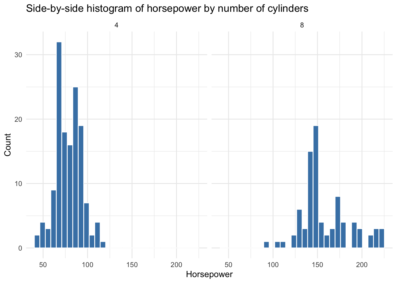

We also look at some descriptive statistics of horsepower in both groups for better understanding of data. The descriptice statistics in cars with 4 cylinders:

summary(train_auto %>% filter(cylinders == 4) %>% select(horsepower))

   horsepower    
 Min.   : 46.00  
 1st Qu.: 68.00  
 Median : 78.00  
 Mean   : 78.47  
 3rd Qu.: 88.00  
 Max.   :115.00

and with 8 cylinders:

summary(train_auto %>% filter(cylinders == 8) %>% select(horsepower))

   horsepower   
 Min.   : 90.0  
 1st Qu.:140.0  
 Median :150.0  
 Mean   :158.8  
 3rd Qu.:175.0  
 Max.   :225.0

Looking at histogram and also summary statistics in different groups we can observe that

Testing Settings

Hypothesis Definitions

Test Flavour and Components

Inferential Conclusions

Storytelling

Ignore the following content for now. Still editting

In this example, we start with a dataset that records the time MDS students spend on course website of DSCI 554. You will encounter this dataset again in DSCI 554 when we discuss A/B/n testing. For now, here’s what the dataset looks like:

ABn_data <- read_csv('data/ABn_data.csv', show_col_types = FALSE)
ABn_data <- ABn_data %>% mutate(Colour = as.factor(Colour), Font = as.factor(Font))
ABn_data

# A tibble: 72 × 3
   Duration Colour Font  
      <dbl> <fct>  <fct> 
 1       90 Red    Small 
 2       95 Red    Large 
 3      107 Red    Medium
 4       92 Red    Small 
 5       89 Red    Large 
 6       92 Red    Medium
 7       81 Red    Small 
 8       92 Red    Large 
 9       93 Red    Medium
10       80 Blue   Small 
# ℹ 62 more rows

The columns in the dataset are as follows:

Font: A factor variable with three levels — small, medium, and large.
Button Colour: A factor variable with two levels — Red and Blue.
Duration: A continuous variable representing the duration of each visit, recorded in minutes.

The main statistical question we are asking here is:

Is there a statistically significant difference in the mean visit duration between websites with red buttons and those with blue buttons?

This means we are interested in the duration time users spend on website in two different populations: red button design and blue button design. First we do some data selection to create two vector of numbers: one for the visit duration visits in website with red buttons and one for the duration of visits in website with blue buttons. The following code can take care of this. For Red group:

duration_red <- ABn_data %>% filter(Colour == 'Red') %>% pull(Duration)
duration_red

 [1]  90  95 107  92  89  92  81  92  93  83  80  95  98  98 106  74  81  74  85
[20]  88  88 112 104  91  82  78  94  86  78  89  79  86  87  85  89  83

and for Blue group:

duration_blue <- ABn_data %>% filter(Colour == 'Blue') %>% pull(Duration)
duration_blue

 [1]  80  87 100 121 110 119  78  98 122 102 109 105  99  94 123 136 133 132  60
[20] 104 114  90 118 113 119 122 136  73 114 114 109 131 126 116 136 133

How to run this test in R?

In order to run this test, similar to what we learned in (LINK to chapter 1) we can use t.test function in R. The function can be used to perform one or two sample t-tests. The relevant arguments of the function are as follows:

x is (non-empty) numeric vector of data values.
y is also (non-empty) numeric vector of data values (can be NULL if you run a one sample test).
var.equal is a binary value (TRUE/FALSE) to indicate if R needs to assume equal variance or not.

Therefore we can run the test for two different cases.

Case 1: Under the assumption that variances between two populations are equal:

t.test(x = duration_red, y = duration_blue, var.equal = TRUE)


    Two Sample t-test

data:  duration_red and duration_blue
t = -6.1183, df = 70, p-value = 4.838e-08
alternative hypothesis: true difference in means is not equal to 0
95 percent confidence interval:
 -28.43489 -14.45400
sample estimates:
mean of x mean of y 
  89.0000  110.4444

Case 2: Under the assumption that variances between two populations are NOT equal:

t.test(x = duration_red, y = duration_blue, var.equal = FALSE)


    Welch Two Sample t-test

data:  duration_red and duration_blue
t = -6.1183, df = 50.043, p-value = 1.429e-07
alternative hypothesis: true difference in means is not equal to 0
95 percent confidence interval:
 -28.48424 -14.40465
sample estimates:
mean of x mean of y 
  89.0000  110.4444

In both outputs, we can see the following:

t is the test statistic.
df is the degrees of freedom for the test.

p-value is the p-value of the test. Note that, by default, this is for a two-sided test. If you need to conduct a one-sided test, you can either divide the p-value by two or use the alternative argument in the t.test function.

95 percent confidence interval provides the 95% confidence interval for \(\mu_1 - \mu_2\).
sample estimates gives the sample means for each group.

Note: By default the value of var.equal is FALSE.

Two sample Welch’s t-test for independent samples

If the assumption of equal variances is questionable, we instead use Welch’s t-test, which adjusts the standard error and degrees of freedom accordingly. The Welch’s test statistic is computed as:

\[t = \frac{\bar{X} - \bar{Y}}{\sqrt{\frac{s_X^2}{n} + \frac{s_Y^2}{m}}}\]

Under the assumption that null hypothesis is correct, the test statistics defined above still follows a t-distribuion but with a different degrees of freedom. The degree of freedom when we do not make equal variance assumption is:

\[\nu = \frac{\left( \frac{s_1^2}{n} + \frac{s_2^2}{m} \right)^2} {\frac{\left( \frac{s_1^2}{n} \right)^2}{n - 1} + \frac{\left( \frac{s_2^2}{m} \right)^2}{m - 1}}\]

Note that this degree of freedom is not necessaily an integer number (could be a real number). When we run t-test, we operate under the assumption that: 1) either the sample size is large enough (we are thinking about \(n=30\) at least) so that central limit theorem assumptions work well, or 2) the distribution of our sample in each group is normal or symmetric enough.

If the normality assumption is also not satisfied (e.g., due to skewed distributions or outliers) or we have a very small sample size, we may turn to a non-parametric alternative, such as the Mann–Whitney–Wilcoxon test, which compares the ranks of the observations across groups rather than the raw values but this book will not cover it. You can read more about it LINK.

Paired Samples

Paired samples arise when each observation in one group is matched or linked to an observation in the other group. This structure is typical in before-and-after studies, matched-subject designs, or repeated measures on the same individuals. A classic example comes from health sciences.

Suppose you’re investigating whether a new diet plan reduces blood pressure. You recruit a group of participants and record their blood pressure before starting the diet. After following the diet for two months, you measure their blood pressure again. In this scenario, each participant contributes two measurements: one before the intervention and one after. These measurements are not independent as they come from the same person. Therefore we treat them as paired.

To formulate the problem and hypothesis, let us assume that each individual has two measurements:

Before the diet: \(X_1, X_2, \ldots, X_n\)
After the diet: \(Y_1, Y_2, \ldots, Y_n\)

Note that in this case the sample size is the same (in both before and after diet sample we have \(n\) observations). We call this a paired sample. Since the samples are paired, we define the difference for each individual as follows:

\[D_i = Y_i - X_i \quad \textit{for} \quad i = 1,2, \ldots, n\] Each \(D_i\) is the difference of blood pressure after and before using new diet. The main statistical question now is:

Is there a statistically significant difference in the mean blood pressure before and after the diet?

In other words, we test the following hypothesis:

\[H_0: \mu_D = 0 \quad \text{versus} \quad H_A: \mu_D \ne 0\] Here the notation of \(\mu_D\) is the population mean of the differences of \(D_i\) which is an unknown parameter in the population. To test this hypothesis, we use the paired t-test, which is essentially a one-sample t-test on the differences \(D_1, D_2, \ldots, D_n\). We test \(\mu_D=0\) because if there is an actual effect of diet on blood pressure, we expect the null hypothesis to be rejected.

The test statistic for this hypothesis testing is:

\[t = \frac{\bar{D}}{s_D / \sqrt{n}}\]