3 Tests for Two Continuous Population Mean

Learning Objectives

By the end of this chapter, you should be able to:

Formulate hypotheses to compare means or proportions in two population.
Choose and conduct appropriate two-sample t-tests or two-proportion z-tests based on study context and assumptions.
Differentiate between independent and paired samples, and choose the appropriate analysis method.
Perform two-sample and paired t-tests and z-test using both R and Python, and interpret the outputs.
Apply statistical reasoning to real-world data examples, including evaluating assumptions and limitations.

This chapter introduces statistical tests designed to compare two samples which is a fundamental task in data analysis across many disciplines. Whether you’re comparing average recovery times between two medical treatments, student test scores under different teaching methods, comparing the proportion among two samples, or reaction times under varying stress conditions, these methods help determine whether observed differences are statistically significant or simply due to chance.

mindmap
  root((Frequentist
  Hypothesis 
  Testings
  ))
    Simulation Based<br/>Tests
    Classical<br/>Tests
      (Chapter 1: <br/>Tests for One<br/>Continuous<br/>Population Mean)
      (Chapter 2: <br/>Tests for Two<br/>Continuous<br/>Population Means)
        Two<br/>Independent<br/>Populations
          {{Unbounded<br/>Responses}}
            Unknown<br/>Population<br/>Variances
              Population<br/>Variances<br/>are assumed<br/>to be Equal
                )Two sample<br/>Student's t test<br/>for Independent<br/>Samples(
              Population<br/>Variances<br/>are assumed<br/>to be Unequal
                )Two sample<br/>Welch's t test<br/>for Independent<br/>Samples(
            Known<br/>Population<br/>Variances
              )Two sample z test<br/>for Independent<br/>Samples(
          {{Proportions between<br/>0 and 1<br/>obtained from two <br/>Binary Responses}}
            )Two sample z test<br/>for Independent<br/>Samples(
        Two<br/>Related<br/>Populations or<br/>Measurements
          {{Unbounded<br/>Responses}}
            )Two sample t test<br/>for Paired<br/>Samples(
      (Chapter 3: <br/>ANOVA-related <br/>Tests for<br/>k Continuous<br/>Population Means)

Figure 3.1: A specific hypothesis testing mind map outlining the techniques explored in this chapter, which are classical tests for two continuous population means.

In this chapter, we review tests for comparing two continuous population means under two conditions: when the populations are independent and when they are dependent. Throughout the sections below, we provide details about these tests and required formula for each case. Broadly speaking, there are two main types of tests to compare the means between two continuous populations:

Independent samples, where the observations in one group are unrelated to those in the other, and
Paired (or dependent) samples, where observations are naturally matched in some way, such as before-and-after measurements.

The choice of test depends on the structure of your data. This chapter introduces both types of comparisons, beginning with independent samples. Each section includes definitions, theoretical background, and R/Python code examples using real or simulated data sets to help ground the concepts in practice. We also review the theoretical background and example codes to test for proportions in two populations.

3.1 Two sample Student’s t-test for Independent Samples

3.1.1 Review

In this section we talk about two sample student’s t-test for independent samples. Independent samples arise when the observations in one group do not influence or relate to the observations in the other. In statistical terms we call this two independent samples. A classic example from educational research is described below:

Suppose you’re interested in whether a new method of teaching introductory physics improves student performance and learning experience. To investigate this, you decide to test the method at two universities: the University of British Columbia (UBC) and Simon Fraser University (SFU). You apply the new teaching method at SFU and compare the results to students taught with the traditional method at UBC.

In this scenario, students at UBC and SFU form two distinct, unrelated groups. Since the students are not paired or matched across schools, and each individual belongs to only one group, the samples are independent. Note that the samples are drawn from two independent population: students at UBC and SFU, respectively.

Let us assume that each population has an unknown average or mean physics score denoted by:

\[ \mu_1 \quad \text{(mean for UBC)}, \quad \mu_2 \quad \text{(mean for SFU)}. \]

Since we do not have access to all students’ grades, we take a random sample from each school. Suppose:

From UBC (Population 1), we obtain a sample of size \(n\), denoted as: \[x_1, x_2, \ldots, x_n\]
From SFU (Population 2), we obtain a sample of size \(m\), denoted as: \[y_1, y_2, \ldots, y_m\]

Note that the sample sizes \(n\) and \(m\) do not necessarily have to be equal. Now, the central question becomes:

Is there a statistically significant difference between the mean physics scores among two groups?

In formal terms, we test the hypotheses:

\[H_0: \mu_1 = \mu_2 \quad \text{versus} \quad H_A: \mu_1 \ne \mu_2\] Now that we reviewed the test concept, let’s try to understand it in a read data set. The steps below follows closely with the roadmap that we introduced in Chapter 1.

3.1.2 Study design

For this example, we will be using Auto data set from ISLR package. This data set contains gas mileage, horsepower, and other information for 392 vehicles. Some of variables of interest are: 1) cylinders an integer (numerical) value between 4 and 8 which indicates the number of cylinders of car, and 2) horsepower which shows engine horsepower. You may wondering if the mean of horsepower in cars with 8 cylinders is statistically different than the means in cars with 4 cylinders?

3.1.3 Data Collection and Wrangling

To answer this question, we obtain the data set which is available in ISLR package. Note that we consider this data a random sample from population of cars. First we create a new copy of this data set to avoid touching the actual data (this is optional). Also we filter rows to those cars with 4 or 8 cylinders only.

# Get a copy of data set
auto_data <- Auto

# Filter rows to cars with 4 or 8 cylinders
auto_data <- auto_data |>  filter(cylinders %in% c(4,8) )

Finally, we randomly create training and test sets from this dataset, using a 50–50 split. It is important to ensure that the proportion of cars with 4 and 8 cylinders remains similar across the two sets; otherwise, the imbalance could introduce bias into our analysis. The initial_split, training, and testing functions from the rsample package are very helpful for handling this correctly.

# Set seed for reproducibility
set.seed(123)

# Randomly splitting into training and testing sets by number of car cylinders
auto_data_splitting <- initial_split(auto_data, prop = 0.5, strata = cylinders)

# Assigning data points to training and testing sets
train_auto <- training(auto_data_splitting)
test_auto  <- testing(auto_data_splitting)

# Sanity check
cat("Training shape:", dim(train_auto), "\n")

Training shape: 150 9

cat("Testing shape:", dim(test_auto), "\n\n")

Testing shape: 152 9

cat("Training proportions:\n")

Training proportions:

print(prop.table(table(train_auto$cylinders)))


   4    8 
0.66 0.34

cat("\nTesting proportions:\n")


Testing proportions:

print(prop.table(table(test_auto$cylinders)))


        4         8 
0.6578947 0.3421053

3.1.4 Explanatory Data Analysis

Once we have the data and it is split into training and test sets, the next step is to begin exploratory data analysis (EDA) on train set. This step is crucial, as it helps us gain a better understanding of the distribution of variables in our data set. The horsepower variable in data set is a numerical variable. The cylinders variable is an integer variable that helps to divide observations into two groups.

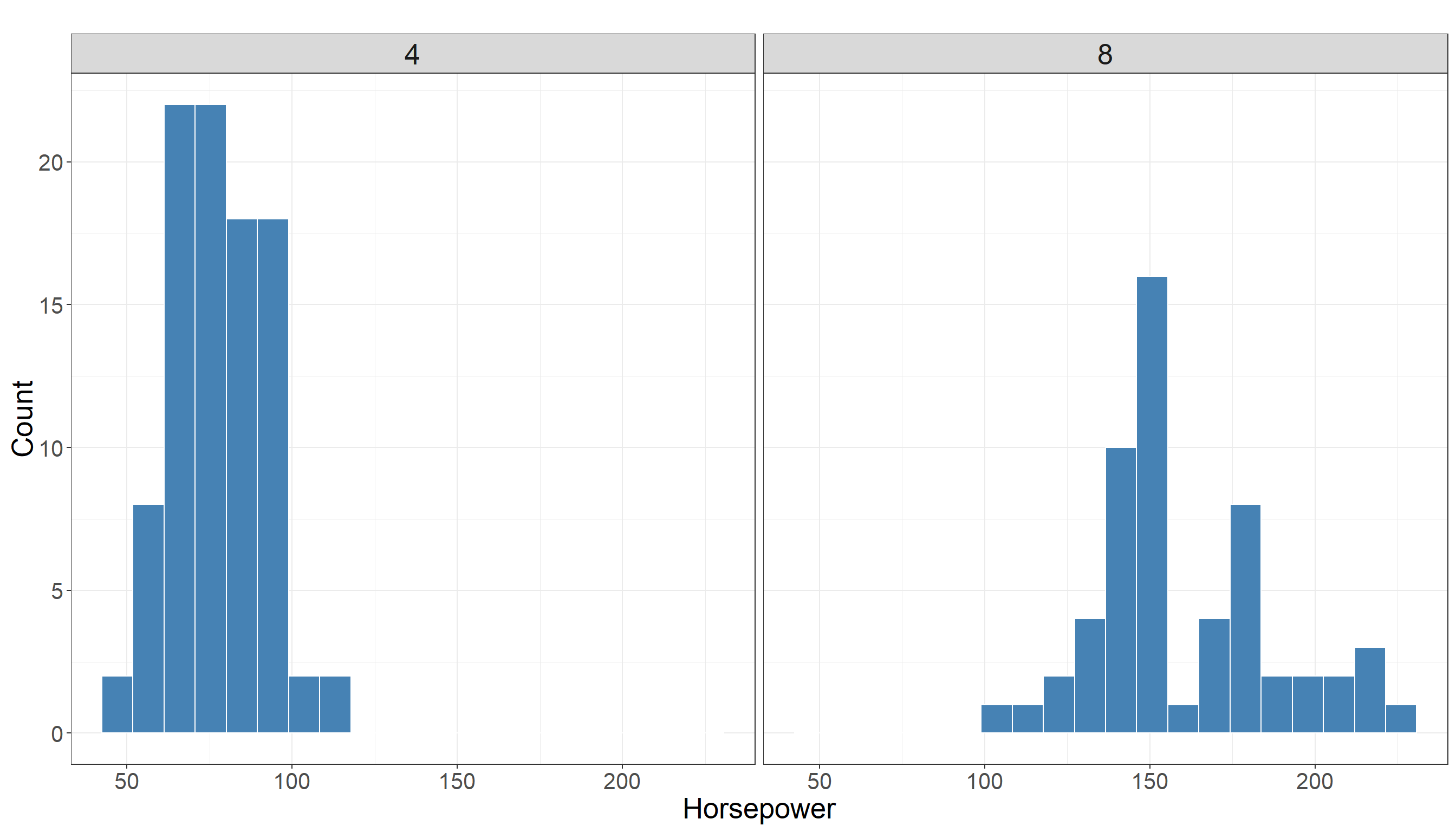
In particular, we are interested in the distribution of horsepower in two different groups (cars with 4 cylinders vs cars with 8 cylinders). Using a histogram for this variable is a good choice as we have a variable with numerical values.

Figure 3.2: Histogram of horsepower by number of cylinders for train data.

We also look at some descriptive statistics of horsepower in both groups for better understanding of data. The descriptive statistics in cars with 4 cylinders:

summary(train_auto |>  filter(cylinders == 4) |>  select(horsepower))

   horsepower    
 Min.   : 46.00  
 1st Qu.: 68.00  
 Median : 80.00  
 Mean   : 79.22  
 3rd Qu.: 90.00  
 Max.   :113.00

and with 8 cylinders:

summary(train_auto |>  filter(cylinders == 8) |>  select(horsepower))

   horsepower   
 Min.   :105.0  
 1st Qu.:140.0  
 Median :150.0  
 Mean   :157.5  
 3rd Qu.:172.5  
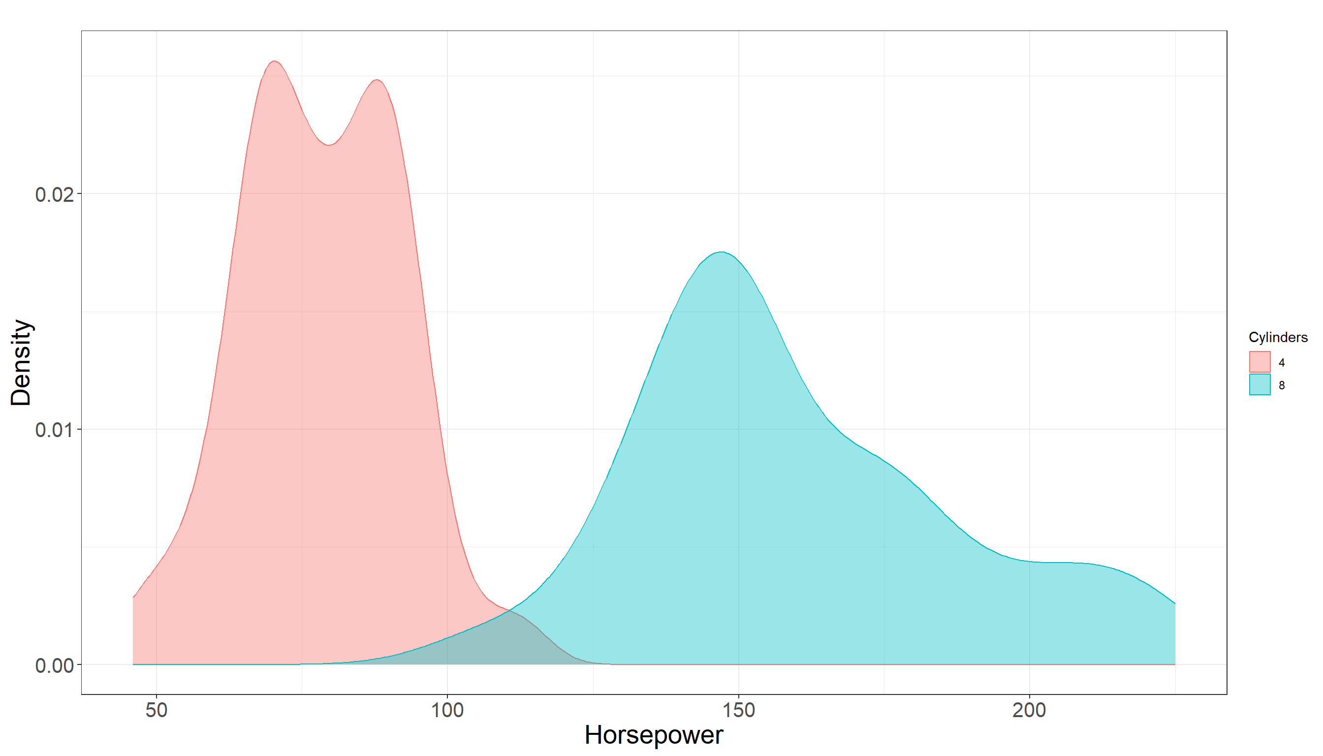
 Max.   :230.0

Looking at summary statistics, there is a bit of overlap between distribution of horsepower among two groups but it does not seem to be much. In fact they seem to be quite separated. Also there is a clear difference in their mean and the following plot also confirms this:

Figure 3.3: Density plot of horsepower by number of cylinders.

3.1.5 Testing Settings

We use a significant level of \(\alpha = 0.05\) to run the test. Considering the data we have is a sample from a population of cars we have the following:

\(\mu_{1}\) is the mean of horsepower for cars with 4 cylinders in the population.
\(\mu_{2}\) is the mean of horsepower for cars with 8 cylinders in the population.

3.1.6 Hypothesis Definitions

We now define the null and alternative hypothesis. Recall the main inquiry we had:

You may wondering if the average of horsepower in cars with 4 cylinders is statistically different than the means in cars with 8 cylinders?

This translates into the following null and alternative hypotheses:

\[H_0: \mu_{1} = \mu_{2} \quad vs \quad H_a: \mu_{1} \neq \mu_{2}\]

Note that the alternative hypothesis is two-sided, as our question does not favor either group and only asks whether the means are different (i.e., group one could be less than or greater than group two). Also the hypothesis tests the unknown parameters in the population which are \(\mu_{1}\) and \(\mu_{2}\).

3.1.7 Test Flavour and Components

To test this hypothesis, we use the two-sample student’s t-test for independent samples, which compares the sample means and incorporates variability within and between the samples. Note that in this case the samples are independent as clearly cars with 4 cylinders are independent from cars with 8 cylinders.

Now we need to compute a test statistic from the sample. Assuming equal population variances, the test statistic is:

\[t = \frac{(\bar{x} - \bar{y})}{ \sqrt{ s^{2}_p (\frac{1}{n} + \frac{1}{m}})} \tag{3.1}\] where:

\(\bar{x}\) is the mean of horsepower for cars with 4 cylinders in the sample
\(\bar{y}\) is the mean of horsepower for cars with 8 cylinders in the sample
\(s^{2}_p\) is the \(\textbf{pooled sample variane}\) and is computed as: \[s^{2}_p = \frac{(n - 1)s_x^2 + (m - 1)s_y^2}{n + m - 2} \tag{3.2}\]
\(s_x^2\) and \(s_y^2\) are the sample variances of the two groups.

Heads-up!

Note that all elements in Equation 3.1 which is our statistic are computed based on sample.
You can think of pooled sample variance defined in Equation 3.2 as a weighted average of sample variances of \(s_x^2\) and \(s_y^2\).
Why it is a weighted average?
The weights are \(\frac{(n - 1)}{n + m - 2}\) and \(\frac{(m - 1)}{n + m - 2}\). These weights reflect how much information each sample’s variance provides — larger samples get more weight. You can see it better if you write it explicitly:

\[ S_p^{2} = \frac{(n - 1)}{n + m - 2} \, s_x^2 + \frac{(m - 1)}{n + m - 2} \, s_y^2 \]

You can see it is literally a weighted mean where weights sum to one:

\[ \frac{n-1}{n+m-2} + \frac{m-1}{n+m-2} = 1 \]

Tip: Equal variance assumption!

The assumption in this test is that variances among two groups in the population are equal meaning that if we look at the random variable of horsepower in both populations, the variance of this random variable is roughly equal in two groups (cars with 4 cylinders and cars with 8 cylinders).
Note that we do not have access to population and this is rather an assumption that we make with consultation with experts or justifying it based on previous studies. We will introduce the test without equal variance assumption in the next section.
There are some statistical methods designed to test if the variances of different groups are the same or not. In fact they can be used to test the equal assumption of variances of groups in the population. Similar to any hypothesis testing, these tests work on a random sample from the population to run the test. Some of the tests are F-test for Equality of Variances, Levene’s Test, and Bartlett’s Test.
Describing these tests is not the focus of this book. You can read more about them HERE/LINK

3.1.8 Inferential Conclusions

As you can see, the test statistic defined in Equation 3.1 computes the difference between \(\bar{x}\) and \(\bar{y}\) and scale it based on the standard deviation of this difference. Now the question is whether this difference is significant or not? In order to answer this question we need to know the behavior of statistic that we defined in Equation 3.1 (and denoted by \(t\)) and have a better understanding of what are typical values of this statistic.

Heads-up!

Note that \(t\) itself is a random variable as it would change from sample to sample.

Knowing the distribution of this statistic helps us to compute \(\textit{p-value}\) of the test as follows:

\[\textit{p-value} = 2 \times Pr(T_{(n+m-2)} \ge |t|)\]

Looking at the formula, we can see that we are essentially calculating how much is it likely to see an observation as big as \(t\) or as extreme as \(t\) (which we computed from our sample) under a t-distribution with a certain degrees of freedom (df) which we are denoting by \(T_{(n+m-2)}\).

Tip:

We skipped the theory behind it but under the assumption that null hypothesis is correct (i.e. \(\mu_1=\mu_2\)) then the test statistic defined in Equation 3.1 (\(t\)) follows a t-distribution with \(n + m -2\) degrees of freedom. We denoted this distribution by \(T_{(n+m-2)}\).
Note: The probability is multiplied by two since we have a two sided hypothesis (alternative is \(\mu_1 \neq \mu_2\)). For a one sided test (when alternative hypothesis is \(\mu_1 > \mu_2\) or \(\mu_1 < \mu_2\)) we do not need to multiply by two.
Now we compare the \(\textit{p-value}\) to our significance level. If the \(\textit{p-value}\) is less than the significance level, then we have evidence against the null hypothesis. The reasoning is as follows: we performed the calculation under the assumption that the null hypothesis is true. If the null hypothesis is true, then the test statistic we computed should follow a \(t\)-distribution with \(n + m - 2\) degrees of freedom. If the p-value is smaller than our chosen significance level, this means it is unlikely that our observed result comes from a \(t\)-distribution with \(n + m - 2\) degrees of freedom. In other words, it is unlikely that our initial assumption about the null hypothesis is correct.

Note that our observation from the sample might still lead us to an incorrect conclusion (since there is variability among samples). Our tolerance for this type of error is determined by the significance level. If \(\textit{p-value}\) is not less than significant level then we do not have any evidence to reject the null hypothesis. Otherwise (if \(\textit{p-value}\) is less than significant level) we do have evidence against the null hypothesis

Now let us see how to run the two-sample test in R and Python. Note that we already used train data for EDA purposes. For the purpose of hypothesis testing now we use test data to avoid double dipping.

3.1.9 How to run the test in `R` and `Python`?

The following lines of code in tabset show you how to run the test in R or Python. Note that generally there are two ways of running this test in R as shown below (there might be other ways but we focus on these two for now). They both give the same result and you are welcome to use either of them. Here is a quick explanation from a coding perspective:

In Option 1, we first select the cars with 4 or 8 cylinders and save each of them in a vector (cylinders_4 and cylinders_8). We then use t.test function to run the test. Note that we pass them as x = cylinders_4 for first group and y = cylinders_8 for the second group.
In Option 2, we use a formula to tell R what is the variable that records the outcome of interest (in this example horsepower variable) and what is the grouping variable (in this example cylinders). This approach is more concise and easier to read, especially when working directly with a data frame. Note that we need to let R know where it can find horsepower and cylinders which we do by setting data = test_auto. Using horsepower ~ cylinders essentially tells R that my varriable of interest for t.test is in horsepower and the grouping variable (4 or 8 cylinders) is in cylinders. Note that the order matters and you can not write it as cylinders ~ horsepower.

# Create a vector to hold horsepower values for cars with 4 cylinders
cylinders_4 <- test_auto |>  filter(cylinders == 4) |>  select(horsepower)

# Create a vector to hold horsepower values for cars with 8 cylinders
cylinders_8 <- test_auto |>  filter(cylinders == 8) |>  select(horsepower)

# Run the test
t.test(x = cylinders_4, y = cylinders_8, var.equal = TRUE)


    Two Sample t-test

data:  cylinders_4 and cylinders_8
t = -23.603, df = 150, p-value < 2.2e-16
alternative hypothesis: true difference in means is not equal to 0
95 percent confidence interval:
 -88.56874 -74.88510
sample estimates:
mean of x mean of y 
  77.3500  159.0769

# Use the formula horsepower ~ cylinders to run the test 
t.test(horsepower ~ cylinders, data = test_auto, var.equal=TRUE)


    Two Sample t-test

data:  horsepower by cylinders
t = -23.603, df = 150, p-value < 2.2e-16
alternative hypothesis: true difference in means between group 4 and group 8 is not equal to 0
95 percent confidence interval:
 -88.56874 -74.88510
sample estimates:
mean in group 4 mean in group 8 
        77.3500        159.0769

from scipy import stats
import pandas as pd

# Read test_auto dataframe in Python as df dataframe
df = pd.read_csv('data/test_auto.csv')

# Select cars with 4 and 8 cylinders
cylinders_4 = df[df["cylinders"] == 4]["horsepower"]
cylinders_8 = df[df["cylinders"] == 8]["horsepower"]

# Run the test
t_stat, p_val = stats.ttest_ind(cylinders_4, cylinders_8, equal_var = True)

# Print t statistic value
print(f"T-statistic: {t_stat}")

T-statistic: -23.6025949975427

# Print p-value of the test
print(f"P-value: {p_val}")

P-value: 2.2949229038881686e-52

Details about R code and output

In order to run this test in R, similar to what we learned in Chapter 2 we can use t.test function in R. The function can be used to perform one or two sample t-tests. The relevant arguments of the function are as follows:

x is (non-empty) numeric vector of data values.
y is also (non-empty) numeric vector of data values (can be NULL if you run a one sample test).
var.equal is a binary value (TRUE/FALSE) to indicate if R needs to assume equal variance between population of two groups or not. By default the value of var.equal is FALSE. We manually set it to TRUE to implement equal variance assumption in our test.

Using Option 1 or Option 2 for R, in both outputs we can see the following elements:

t is the test statistic defined in Equation 3.1
df is the degrees of freedom for the test. You can manually calculate and confirm/see that it equals \(n+m-2\).
p-value is the \(\textit{p-value}\) of the test. Note that, by default, this is for a two-sided test. If you need to conduct a one-sided test, you can either divide the p-value by two or use the alternative argument in the t.test function. You can read more about it in help documentation of t.test function (type and run help(t.test) in R console and look for alternative argument.)
95 percent confidence interval provides the 95% confidence interval for the parameter of \(\mu_1 - \mu_2\). You can control the level of your confidence interval by setting conf.level to other values between 0 and 1. By default it is set to conf.level = 0.95.
sample estimates gives the sample means for each group, i.e. \(\bar{x}\) and \(\bar{y}\).

Details about Python code and output

In this example, we perform the test in Python. We use pandas package to read data in Python and scipy for running the test. Here is a breakdown of key points:

cylinders_4 and cylinders_8 are pandas objects containing the horsepower values for cars with 4 and 8 cylinders, respectively.
The function ttest_ind from stats module computes the t-test for the means of two independent samples.
The argument equal_var=True tells Python to assume equal population variances (similar to setting var.equal = TRUE in t.test function R).
The function returns two values: t_stat which is the computed t-statistic and p_val which is the \(\textit{p-value}\) of the test. By default, ttest_ind performs a two-sided test. For a one-sided test, you would need to adjust the \(\textit{p-value}\) accordingly (e.g., divide by two if the t-statistic is in the direction of interest).
This Python approach is directly comparable to using t.test in R, with the main conceptual difference being how arguments are named and handled.

3.1.10 Storytelling

Finally, based on the sample we have and the analysis we conducted, we can draw a conclusion about our initial question: Is the mean horsepower of cars with 8 cylinders statistically different from that of cars with 4 cylinders?

We observed that the \(p-\textit{value}\) of the test was extremely small compared to the significance level \(\alpha = 0.05\). This provides strong evidence against the null hypothesis. In simple terms, this means: There is a meaningful difference in the average horsepower between cars with 4 cylinders and those with 8 cylinders.

So, if you are shopping for a car with more horsepower, it looks like going for one with 8 cylinders might be the way to go as you get a significant boost in powerhorse — assuming you don’t mind the extra fuel costs of course!!

3.2 Two sample Welch’s t-test for independent samples

3.2.1 Review

In this section, we discuss the two-sample Welch’s t-test for independent samples. This test is similar to the two-sample Student’s t-test we described earlier in Section 3.1, with one important difference: it does not assume equal variances between the two groups. We use the Welch’s t-test when we have no reason or evidence to believe that the variable of interest has the same variance in both population groups.

3.2.2 Study Design

We will be using Auto data set from ISLR package in this section too. Now the main statistical question of interest remains the same as before: You may wondering if the mean of horsepower in cars with 8 cylinders is statistically different than the means in cars with 4 cylinders? but we do not make an equal variance assumption anymore.

In this context, unequal variances mean that the spread or variability of horsepower values could differ between the two groups, so we allow each group to have its own variance estimate. Now we are applying a two sample Welch’s t-test for independent samples.

3.2.3 Data Collection and Wrangling

To answer the question, we obtain the data set which is available in ISLR package. The following codes are exactly the same as described in Data Collection and Wrangling of Section 3.1 and are shown here as a review. Essentially the data sets (train and test) that we use in this section are the same as previous example.

# Get a copy of data set
auto_data <- Auto

# Filter rows to cars with 4 or 8 cylinders
auto_data <- auto_data |>  filter(cylinders %in% c(4,8) )

# Set seed for reproducibility
set.seed(123)

# Randomly splitting into training and testing sets by number of car cylinders
auto_data_splitting <- initial_split(auto_data, prop = 0.5, strata = cylinders)

# Assigning data points to training and testing sets
train_auto <- training(auto_data_splitting)
test_auto  <- testing(auto_data_splitting)

# Sanity check
cat("Training shape:", dim(train_auto), "\n")
cat("Testing shape:", dim(test_auto), "\n\n")
cat("Training proportions:\n")
print(prop.table(table(train_auto$cylinders)))
cat("\nTesting proportions:\n")
print(prop.table(table(test_auto$cylinders)))

3.2.4 Explanatory Data Analysis

Once we have the data and it is split into training and test sets, the next step is to begin exploratory data analysis (EDA) on train set. Recall that the cylinders variable is an integer variable that helps to divide observations into two groups.

We are still interested in the distribution of horsepower in two different groups (cars with 4 cylinders vs cars with 8 cylinders). Using a histogram for this variable is a good choice as we have a variable with numerical values. The following plot is the same as before and we are showing it here as a review.

Figure 3.4: Histogram of horsepower by number of cylinders for train data.

The descriptive statistics in cars with 4 cylinders:

summary(train_auto |>  filter(cylinders == 4) |>  select(horsepower))

   horsepower    
 Min.   : 46.00  
 1st Qu.: 68.00  
 Median : 80.00  
 Mean   : 79.22  
 3rd Qu.: 90.00  
 Max.   :113.00

and with 8 cylinders:

summary(train_auto |>  filter(cylinders == 8) |>  select(horsepower))

   horsepower   
 Min.   :105.0  
 1st Qu.:140.0  
 Median :150.0  
 Mean   :157.5  
 3rd Qu.:172.5  
 Max.   :230.0

Our conclusion remains the same. Looking at summary statistics, there is a bit of overlap between distribution of horsepower among two groups but it does not seem to be much. In fact they seem to be quite separated. Also there is a clear difference in their mean and the following plot also confirms this:

Figure 3.5: Density plot of horsepower by number of cylinders.

3.2.5 Testing Settings

We use a significant level of \(\alpha = 0.05\) to run the test. Considering the data we have is a sample from a population of cars we have the following parameters of interset in our population:

\(\mu_{1}\) is the mean of horsepower for cars with 4 cylinders in the population.
\(\mu_{2}\) is the mean of horsepower for cars with 8 cylinders in the population.

3.2.6 Hypothesis Definitions

We now define the null and alternative hypothesis. Recall the main inquiry we had:

You may wondering if the average of horsepower in cars with 4 cylinders is statistically different than the means in cars with 8 cylinders?

This translates into the following null and alternative hypotheses:

\[H_0: \mu_{1} = \mu_{2} \quad vs \quad H_a: \mu_{1} \neq \mu_{2}\]

3.2.7 Test Flavour and Components

As noted before we use Welch’s t-test if the assumption of equal variances is questionable. This test adjusts the standard error and degrees of freedom (df) of the test accordingly. As a result the test statistic and df of the test are different than what we described in Section 3.1. The Welch’s test statistic is computed as:

\[t = \frac{\bar{x} - \bar{y}}{\sqrt{\frac{s_x^2}{n} + \frac{s_y^2}{m}}} \tag{3.3}\]

where:

\(\bar{x}\) is the mean of horsepower for cars with 4 cylinders in the sample
\(\bar{y}\) is the mean of horsepower for cars with 8 cylinders in the sample
\(s_x^2\) and \(s_y^2\) are the sample variances of the two groups.
\(n\) and \(m\) are the sample sizes in two groups (not necessarily the same).

Quick review!

Note that, as before, all elements in Equation 3.3 (statistic) are computed based on the sample.
Additionally, the assumption of unequal variance between two populations can be tested using a variety of statistical tests.
We do not discuss these tests in this book as the focus of this book lies elsewhere. If you are interested to read more about it, refer to REF.

3.2.8 Inferential Conclusions

As you can see, the test statistic in Equation 3.3 computes the difference between averages of two samples and adjusts it based on the standard deviation of their differences. The only change from Student’s t-test is the standard deviation that is being used in the denominator. Again the question is whether this difference is significant or not?

In order to answer this question we need to know the behavior of statistic that we defined in Equation 3.3 and have a better understanding of what are typical values of this statistic. Knowing the distribution of this statistic helps us to compute the \(\textit{p-value}\) of the test as follows:

\[\textit{p-value} = 2 \times Pr(T_{\nu} \ge |t|)\]

Tip on degrees of freedom!

We skipped the theory behind it but under the assumption that null hypothesis is correct, it can be shown that the test statistic defined in Equation 3.3 still follows a t-distribution but with a different degrees of freedom (df).
Note that this degree of freedom is not necessarily an integer number (could be a real number).
The Greek sign \(\nu\) is used here to show the degree of freedom of t-distribution shown in \(T_{\nu}\).
The degree of freedom is computed as

\[\nu = \frac{\left( \frac{s_x^2}{n} + \frac{s_y^2}{m} \right)^2} {\frac{\left( \frac{s_x^2}{n} \right)^2}{n - 1} + \frac{\left( \frac{s_y^2}{m} \right)^2}{m - 1}}\]

3.2.9 How to run the test in `R` and `Python`?

The following lines of code in tabset show you how to run the Welch’s test in R or Python.

A quick reminder!

In Option 1, we first select the cars with 4 or 8 cylinders and save them in a vector (cylinders_4 and cylinders_8). We then use t.test function to run the test.
In Option 2, we use a formula to tell R what is the variable that records the outcome of interest (in this example horsepower variable) and what is the grouping variable (in this example cylinders).
Using Option 2 is more concise and easier to read, especially when working directly with a data frame.
Note that we need to let R know where it can find horsepower and cylinders which we do by setting data = test_auto.

# Create a vector to hold horsepower values for cars with 4 cylinders
cylinders_4 <- test_auto |> filter(cylinders == 4) |> select(horsepower)

# Create a vector to hold horsepower values for cars with 8 cylinders
cylinders_8 <- test_auto |> filter(cylinders == 8) |> select(horsepower)

# Run the test
t.test(x = cylinders_4, y = cylinders_8, var.equal = FALSE)


    Welch Two Sample t-test

data:  cylinders_4 and cylinders_8
t = -19.37, df = 64.007, p-value < 2.2e-16
alternative hypothesis: true difference in means is not equal to 0
95 percent confidence interval:
 -90.15599 -73.29786
sample estimates:
mean of x mean of y 
  77.3500  159.0769

# Use the formula horsepower ~ cylinders to run the test 
t.test(horsepower ~ cylinders, data = test_auto, var.equal = FALSE)


    Welch Two Sample t-test

data:  horsepower by cylinders
t = -19.37, df = 64.007, p-value < 2.2e-16
alternative hypothesis: true difference in means between group 4 and group 8 is not equal to 0
95 percent confidence interval:
 -90.15599 -73.29786
sample estimates:
mean in group 4 mean in group 8 
        77.3500        159.0769

from scipy import stats
import pandas as pd

# Read test_auto dataframe in Python as df dataframe
df = pd.read_csv('data/test_auto.csv')

# Select cars with 4 and 8 cylinders
cylinders_4 = df[df["cylinders"] == 4]["horsepower"]
cylinders_8 = df[df["cylinders"] == 8]["horsepower"]

# Run the test
t_stat, p_val = stats.ttest_ind(cylinders_4, cylinders_8, equal_var = False)

# Print t statistic value
print(f"T-statistic: {t_stat}")

T-statistic: -19.36963609727327

# Print p-value of the test
print(f"P-value: {p_val}")

P-value: 1.8268539721413396e-28

Details about R code and output

x is (non-empty) numeric vector of data values.
y is also (non-empty) numeric vector of data values (can be NULL if you run a one sample test).
var.equal is a binary value (TRUE/FALSE) to indicate if R needs to assume equal variance between population of two groups or not. By default the value of var.equal is FALSE but we manually set it to FALSE to make it clear to the reader that we are making an unequal variance assumption in our test.

Using Option 1 or Option 2 for R, in both outputs we can see the following elements:

t is the test statistic defined in Equation 3.3
df is the degrees of freedom for the test. You can manually calculate and confirm/see that it equals \(\nu\) that we defined in Equation 3.3.
p-value is the \(\textit{p-value}\) of the test. Note that, by default, this is for a two-sided test. If you need to conduct a one-sided test, you can either divide the p-value by two or use the alternative argument in the t.test function. You can read more about it in help documentation of t.test function (type and run help(t.test) in R console and look for alternative argument.)
95 percent confidence interval provides the 95% confidence interval for the parameter of \(\mu_1 - \mu_2\). You can control the level of your confidence interval by setting conf.level to other values between 0 and 1. By default it is set to conf.level = 0.95.
sample estimates gives the sample means for each group, i.e. \(\bar{x}\) and \(\bar{y}\).

Details about Python code and output

In this example, we perform the test in Python. We use pandas package to read data in Python and scipy for running the test. Here is a breakdown of key points:

cylinders_4 and cylinders_8 are pandas objects containing the horsepower values for cars with 4 and 8 cylinders, respectively.
The function ttest_ind from stats module computes the t-test for the means of two independent samples.
The argument equal_var=False tells Python to assume unequal population variances (similar to setting var.equal = FALSE in t.test function R).
The function returns two values: t_stat which is the computed t-statistic and p_val which is the \(\textit{p-value}\) of the test. By default, ttest_ind performs a two-sided test. For a one-sided test, you would need to adjust the \(\textit{p-value}\) accordingly (e.g., divide by two if the t-statistic is in the direction of interest).
This Python approach is directly comparable to using t.test in R, with the main conceptual difference being how arguments are named and handled.

3.2.10 Storytelling

So, if you are shopping for a car with more horsepower, it looks like going for one with 8 cylinders might be the way to go — assuming you don’t mind the extra fuel costs of course!!

3.3 Two sample z-test for Independent Samples

3.3.1 Review

In the tests we have seen so far in Section 3.1 and Section 3.2, we estimated the variance of each group using the sample variance. For example see \(s^2_{x}\) or \(s^2_{y}\) defined in formula Equation 3.3. This approach is realistic, as in most cases we do not know the population variance of our variable of interest and it is being estimated by sample variance. However, if the population variance for each group is known we can incorporate this information into our test.

For example, suppose you are analyzing wage differences between high school and college graduates using a large labor market data set. A government labor agency previously conducted extensive research and reported that the true population variances of hourly wages for both groups (based on some historical data) should be as follows:

Population variance of wages among high school graduates: \(\sigma_1^2 = 816\)
Population variance of wages among college graduates: \(\sigma_2^2 = 1700\)

Note that this is the population variance and not the sample. You want to assess whether the average wage differs between the two groups. Since the population variances are known (e.g., from reliable historical studies or large scale sampling in previous studies), a two-sample z-test is appropriate instead of a t-test. We treat these groups as independent samples since each person’s wage is recorded once and belongs to a distinct education level.

Since we do not have access to the wages of all individuals in each education group, we take a random sample from each population. Suppose:

From the population of high school graduates (Population 1), we obtain a sample of size \(n\), denoted as:

\[x_1, x_2, \ldots, x_n\]

From the population of college graduates (Population 2), we obtain a sample of size \(m\), denoted as:

\[y_1, y_2, \ldots, y_m\] Note that the sample sizes \(n\) and \(m\) do not need to be equal. Now, the central question becomes Is there a statistically significant difference between the mean wages of high school and college graduates? In formal terms, we test the hypotheses:

\[ H_0: \mu_1 = \mu_2 \quad \text{versus} \quad H_A: \mu_1 \ne \mu_2 \] where \(\mu_1\) is the population mean of wage in high school graduates and \(\mu_2\) is the population mean of wage in college graduates.

3.3.2 Study Design

For this example, we will be using the Wage data set from the ISLR2 package. This data set contains information about wages and demographic characteristics for 3,000 workers in the Mid-Atlantic region of the United States. Some of the variables of interest are:

education, a categorical variable that records the highest level of education completed by the individual (e.g., “HS Grad”, “College Grad”), and
wage, which denotes the workers raw wage.

You may be wondering: Is the mean wage for college graduates statistically different from the mean wage for high school graduates?

To answer this question, we will compare the sample means of these two groups using a two-sample z-test under the assumption that the population variances are known. We use the Wage data set to extract wage data for two groups:

High school graduates: education == "HS Grad"
College graduates: education == "College Grad"

3.3.3 Data Collection and Wrangling

To answer this question, we obtain the data set which is available in the ISLR2 package. Note that we consider this data a random sample from the population of working adults. First, we create a new copy of this data set to avoid modifying the original data (this step is optional). Then, we filter the rows to keep only individuals who are either high school graduates or college graduates.

# Get a copy of data set
wage_data <- Wage

# Filter rows to keep only HS Grad and College Grad 
# and then rename the levels to:
# - HS Grad --> High school graduate
# - College Grad --> College graduate
# and finally drop extra levels from education
wage_data <- wage_data |> 
  filter(education %in% c('2. HS Grad', '4. College Grad')) |> 
  mutate(education = recode(education,
                            '2. HS Grad' = 'High school graduate',
                            '4. College Grad' = 'College graduate')) |>
  mutate(education = droplevels(education))

Finally, we randomly split the wage_data data set into training and testing sets, using a 50-50 proportion between train and test following a similar method as we described earlier. This allows us to conduct our test using a subset of the data (train) while reserving the rest (test) for potential follow-up analysis.

# Set seed for reproducibility
set.seed(123)

# Randomly splitting into training and testing sets by level of education
wage_data_splitting <- initial_split(wage_data, prop = 0.5, strata = education)

# Assigning data points to training and testing sets
train_wage <- training(wage_data_splitting)
test_wage  <- testing(wage_data_splitting)

# Sanity check
cat("Training shape:", dim(train_wage), "\n")

Training shape: 827 11

cat("Testing shape:", dim(test_wage), "\n\n")

Testing shape: 829 11

cat("Training proportions:\n")

Training proportions:

print(prop.table(table(train_wage$education)))


High school graduate     College graduate 
           0.5864571            0.4135429

cat("\nTesting proportions:\n")


Testing proportions:

print(prop.table(table(test_wage$education)))


High school graduate     College graduate 
           0.5862485            0.4137515

3.3.4 Exploratory Data Analysis

Once we have the data and it is split into training and test sets, the next step is to begin exploratory data analysis (EDA) on the training set. The wage variable is a numerical variable that represents hourly earnings. The education variable is a categorical variable that helps us divide observations into two groups.

In particular, we are interested in the distribution of wage in two different groups (high school graduates vs college graduates). Using a histogram for this variable is a good choice as it allows us to visually inspect how the wages vary within and between these two education levels.

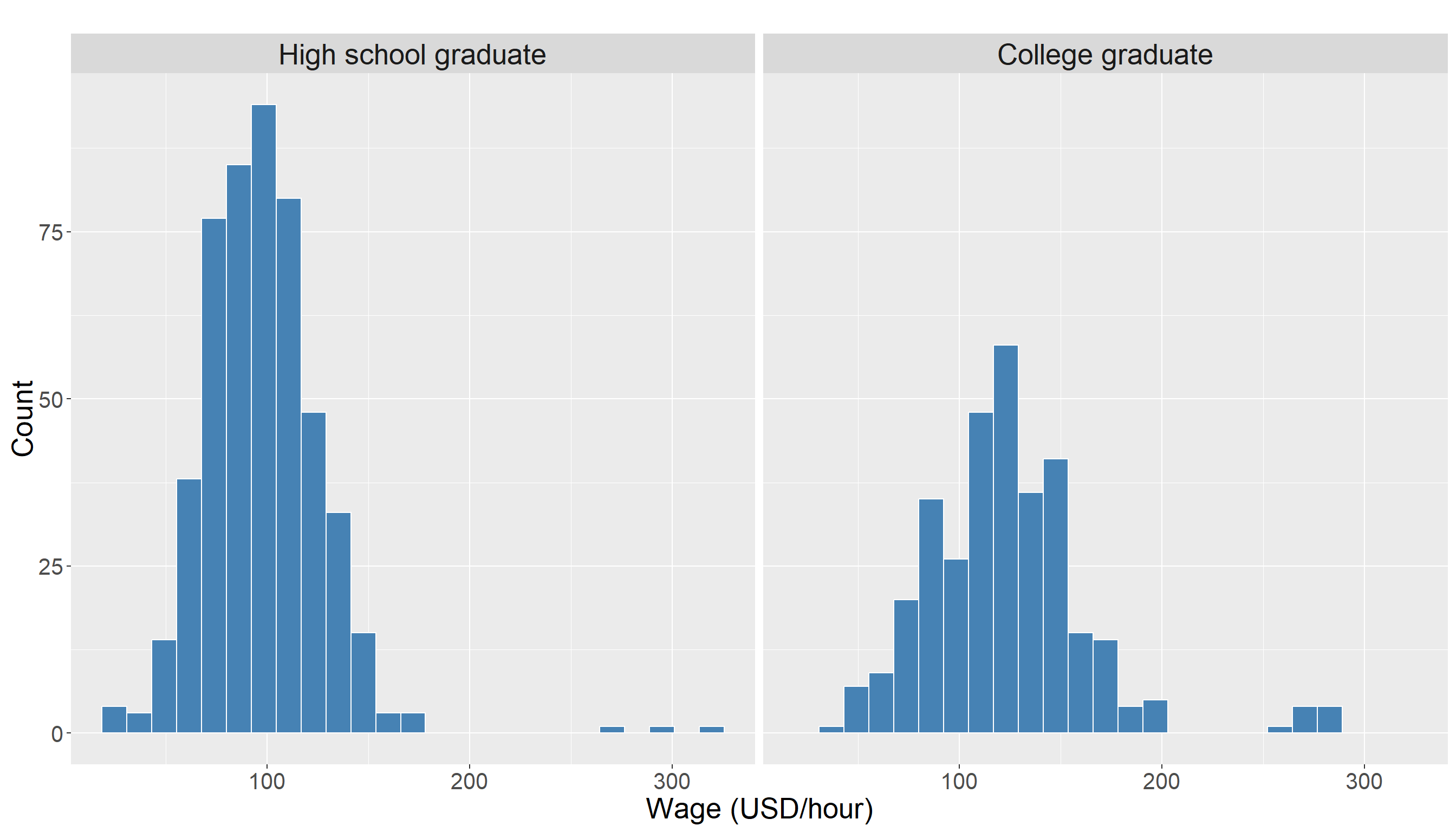
Figure 3.6: Hsistogram of wage by education level

We also look at some descriptive statistics of wage in both groups for better understanding of the data. The descriptive statistics for high school graduates:

summary(train_wage |> 
          filter(education == 'High school graduate') |> 
          select(wage))

      wage       
 Min.   : 27.14  
 1st Qu.: 78.39  
 Median : 92.90  
 Mean   : 95.27  
 3rd Qu.:109.83  
 Max.   :295.99

and for college graduates:

summary(train_wage |> 
          filter(education == 'College graduate') 
        |> select(wage))

      wage       
 Min.   : 34.61  
 1st Qu.: 98.87  
 Median :118.72  
 Mean   :121.44  
 3rd Qu.:141.43  
 Max.   :277.80

Looking at these summary statistics, we can see that the wage distributions for the two education groups have quite a lot of overlap, and there does not appear to be a large difference in the center of distribution In fact, the mean wage for college graduates is only slightly higher, and this is not immediately obvious from the plots.

There appears to be some observations with higher wage values in College Grad group compared to High School Graduate. The following density plot provides additional visual support for this observation:

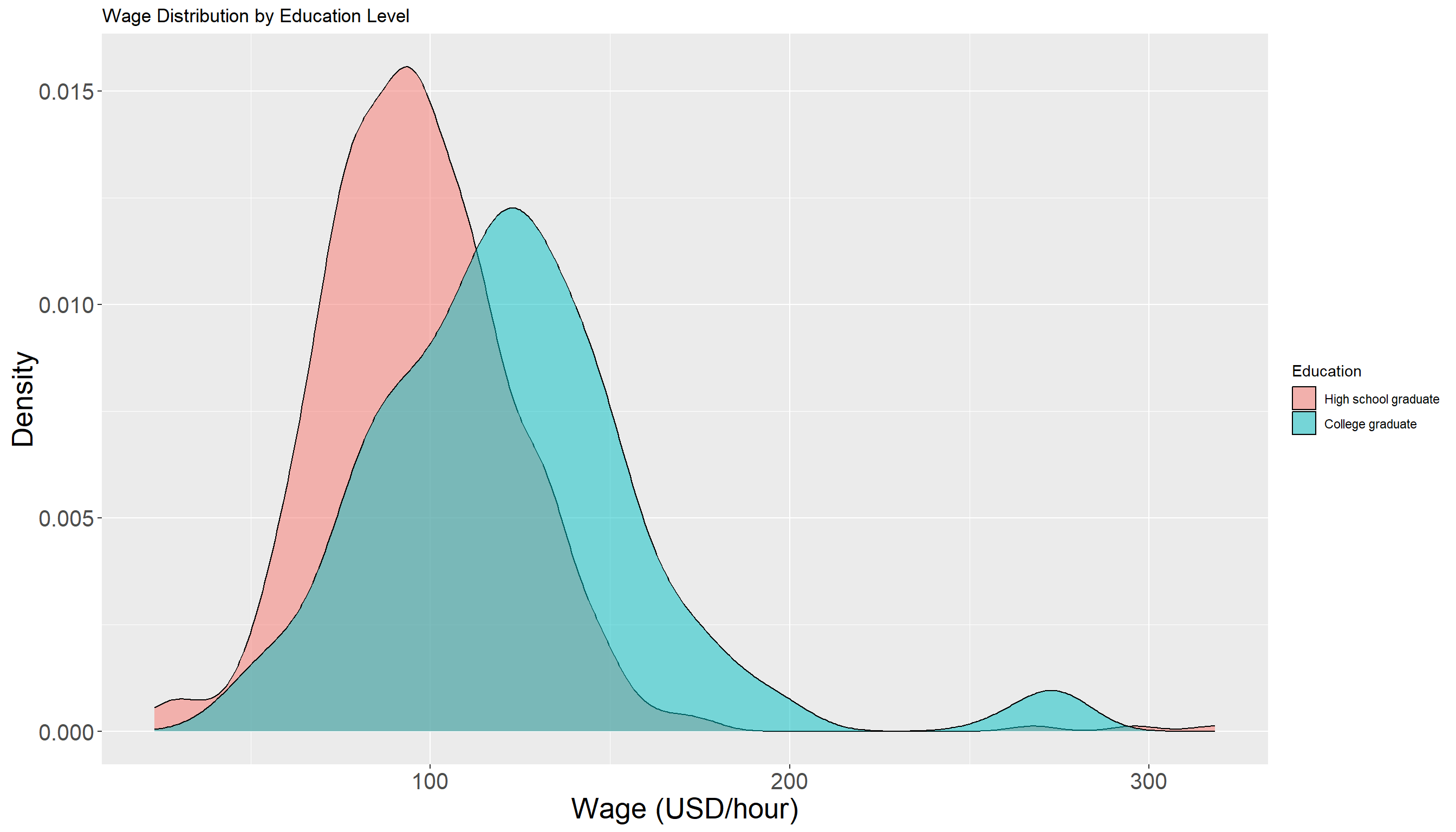
Figure 3.7: Density plot of wage by education level.

We should avoid making any firm conclusion from EDA at this step. The density of both groups seems to have some overlap but in order to answer our initial question, we need to perform a formal hypothesis testing to see if the observed difference is indeed significant or not.

3.3.5 Testing Settings

We use a significance level of \(\alpha = 0.05\) to conduct the hypothesis test. Since the data we have is a sample from a larger population of workers, we define the following population parameters:

\(\mu_{1}\) is the mean wage of individuals with a high school education in the population.
\(\mu_{2}\) is the mean wage of individuals with a college education in the population.

Our goal is to test whether the population mean wage differs between these two educational groups.

3.3.6 Hypothesis Definitions

We now define the null and alternative hypothesis. Recall the main inquiry we had:

Is the mean wage for college graduates statistically different from the mean wage for high school graduates?

This translates into the following null and alternative hypotheses:

\[H_0: \mu_{1} = \mu_{2} \quad vs \quad H_a: \mu_{1} \neq \mu_{2}\]

3.3.7 Test Flavour and Components

To test this hypothesis, we use the two-sample z-test for independent samples with known population variances, which compares the sample means and incorporates the known variability within each population. Note that the samples are independent. The test statistic for this test is computed as:

\[z = \frac{\bar{x} - \bar{y}}{\sqrt{\frac{\sigma_1^2}{n} + \frac{\sigma_2^2}{m}}} \tag{3.4}\]

where:

\(\bar{x}\) is the mean wage of individuals with a high school education in the sample.
\(\bar{y}\) is the mean wage of individuals with a college education in the sample.
\(\sigma_1^2\) and \(\sigma_2^2\) are the known population variances of the two groups
\(n\) and \(m\) are the sample sizes of the two groups

Because population variances are known, the standard error of the difference in sample means is computed directly from the population variances, avoiding the need to estimate variance from the samples.

Heads-up!

Note that \(z\) defined in Equation 3.4 itself is a random variable meaning that it would vary from sample to sample.

3.3.8 Inferential Conclusions

As you can see, the test statistic defined in Equation 3.4 computes the difference between \(\bar{x}\) and \(\bar{y}\) and scales it based on the known variance of this difference (or more precisely standard deviation of the difference!). Now the question is whether this difference is significant or not? To answer this, we need to understand the behavior of the statistic we defined in Equation 3.4 (\(z\)) and what typical values it can take.

As we shown before, knowing the distribution of this statistic allows us to compute the \(\textit{p-value}\) of the test as follows:

\[\textit{p-value} = 2 \times Pr(Z \ge |z|) \tag{3.5}\]

Upper case \(Z\) vs lower case \(z\)!

The lower case \(z\) in Equation 3.5 is the statistic computed from the sample (Equation 3.4).
The upper case \(Z\) though is a notation to use for random variable.
This random variable follows a Normal distribution with mean zero and standard deviation of one.
Looking at the formula in Equation 3.5, we are essentially calculating how likely it is to observe a value as extreme as \(z\) under the null hypothesis - a Normal distribution with mean zero and standard deviation of one.

Interpreting the Test Statistic and p-value!

Under the assumption that the null hypothesis is correct (i.e., \(\mu_1 = \mu_2\)), the test statistic \(z\) follows the standard normal distribution that textbooks usually denote it by \(N(0,1)\). The first element is mean (0) and the second one is the standard deviation (1).
Note: The probability is multiplied by two because we are conducting a two-sided test (alternative hypothesis: \(\mu_1 \neq \mu_2\)). For a one-sided test (e.g., \(\mu_1 > \mu_2\) or \(\mu_1 < \mu_2\)) this multiplication is not needed.
We compare the \(\textit{p-value}\) to our significance level \(\alpha\). If the \(\textit{p-value}\) is less than \(\alpha\), then we have evidence against the null hypothesis.
The reasoning is: assuming the null hypothesis is true, the test statistic should follow a standard normal distribution. A very small \(\textit{p-value}\) means our observed \(z\) is unlikely under this distribution, and so it is unlikely the null hypothesis is correct.

3.3.9 How to run the two-sample `z-test` in `R` and `Python`

The following examples show how to implement the two-sample z-test for independent samples with known population variances in both R and Python using the Wage data set. Note that we know the population variances \(\sigma_1^2 = 816\) for high school graduates and \(\sigma_2^2 = 1700\) for college graduates.

R Code
Python Code

# Filter test_wage data to create two groups: 
# High school graduates and college graduates
hs_wages <- test_wage |> 
  filter(education == 'High school graduate') |> 
  pull(wage)

col_wages <- test_wage |> 
  filter(education == 'College graduate') |> 
  pull(wage)

# Set the known population variances
sigma2_hs <- 816
sigma2_col <- 1700

# Run two-sample z-test with known variances
result <- z.test(
  x = hs_wages,
  y = col_wages,
  sigma.x = sqrt(sigma2_hs),  # standard deviation for group 1
  sigma.y = sqrt(sigma2_col), # standard deviation for group 2
  alternative = "two.sided"
)

# Print results
print(result)


    Two-sample z-Test

data:  hs_wages and col_wages
z = -12.079, p-value < 2.2e-16
alternative hypothesis: true difference in means is not equal to 0
95 percent confidence interval:
 -36.16323 -26.06588
sample estimates:
mean of x mean of y 
 96.29123 127.40579

import pandas as pd
import numpy as np
from scipy.stats import norm


# Read data set
df = pd.read_csv('data/test_wage.csv')

# Extract wages for high school graduates and college graduates
hs_wages = df.loc[df['education'] == 'High school graduate', 'wage'].to_numpy()
col_wages = df.loc[df['education'] == 'College graduate', 'wage'].to_numpy()

# Sample sizes
n1 = len(hs_wages)
n2 = len(col_wages)

# Sample means
mean1 = np.mean(hs_wages)
mean2 = np.mean(col_wages)

# Standard deviations (square root of known variances)
sigma1 = np.sqrt(816)
sigma2 = np.sqrt(1700)

# Calculate standard error using known population std dev
se = np.sqrt( (sigma1**2 / n1) + (sigma2**2 / n2) )

# Calculate z-statistic
z_stat = (mean1 - mean2) / se

# Two-sided p-value
p_value = 2 * norm.cdf(-abs(z_stat))

# Print z-statistic and p-value
print(f"Z-statistic: {z_stat}")

Z-statistic: -12.079082633142994

print(f"P-value: {p_value}")

P-value: 1.3623112108098036e-33

In order to run the two-sample z-test with known population variances, we use the z.test function from the BSDA package in R which have a similar input and output to t.test function. This function is designed to handle one and two sample z-tests when population standard deviations are known. The key arguments of z.test for a two-sample test are:

x: a numeric vector of data values for group 1.
y: a numeric vector of data values for group 2.
sigma_x: the known population standard deviation for group 1.
sigma_y: the known population standard deviation for group 2.
alternative: specifies the alternative hypothesis; "two.sided" by default for a two-sided test.

Note: sigma_x and sigma_y expects the standard deviation of each group and not the variance. As a result in the R code in tabset we passed sqrt(sigma2_hs) and sqrt(sigma2_col).

When you run the test, the output includes:

statistic: the calculated \(z\) test statistic defined in Equation 3.4.
p.value: the p-value for the test based on the standard normal distribution, defined in Equation 3.5.
conf.int: the confidence interval for the difference in means \(\mu_1 - \mu_2\).
estimate: the sample means for each group.

Note: The z.test function assumes that the population standard deviations are known and uses them directly to compute the test statistic and confidence interval. This differs from tests that estimate variance from the samples such as t-tests that we discussed in Section 3.1 and Section 3.2.

3.3.10 Storytelling

In summary, these results tell us that the observed difference in wages is highly unlikely to have occurred by random chance if the true means were equal. Therefore, we conclude that college graduates earn significantly more than high school graduates on average.

3.4 Two sample t-test for Paired Samples

3.4.1 Review

In this section, we discuss the two sample t-test for paired samples which is used when we have two sets of related observations. Unlike the two-sample t-tests for independent samples that we discussed so far (such as the Student’s or Welch’s t-test), the paired t-test is appropriate when the two samples are dependent. This means each observation in one sample can be naturally paired with an observation in the other.

Examples of such are before-and-after measurements on the same subjects, or matched subjects across two different conditions. The key idea is that the test evaluates whether the mean difference between paired observations is significantly different from zero.

When to use this test!

We use the paired sample t-test when:

The data consist of paired observations.
The differences between pairs are approximately normally distributed or at least symmetric (especially important for small sample sizes).
And the measurement scale is continuous.

Paired samples arise when each observation in one group is matched or linked to an observation in the other group. This structure is typical in before-and-after studies, matched-subject designs, or repeated measures on the same individuals. A classic example comes from health sciences.

Suppose you are investigating whether a new diet plan reduces blood pressure. You recruit a group of participants and record their blood pressure before starting the diet. After following the diet for two months, you measure their blood pressure again. In this scenario, each participant contributes two measurements: one before the intervention and one after. Note that these measurements are not independent as they come from the same person. Therefore we treat them as paired.

To formulate the problem and hypothesis, let us assume that each individual has two measurements:

Before the diet: \(x_1, x_2, \ldots, x_n\)
After the diet: \(y_1, y_2, \ldots, y_n\)

Note that in this case the sample size is the same (in both before and after diet sample we have \(n\) observations). We call this a paired sample. Since the samples are paired, we define the difference for each individual as follows:

\[d_i = y_i - x_i \quad \textit{for} \quad i = 1,2, \ldots, n\] Each \(d_i\) is the difference of blood pressure after and before using new diet for the \(i\)-th person. Now the main statistical question is:

Is there a significant difference in the mean blood pressure before and after the diet?

Now if the treatment is effective, one expect to have difference sample average of around zero. In other words, we test the following hypothesis:

\[H_0: \mu_d = 0 \quad \text{versus} \quad H_A: \mu_d \ne 0\]

where \(\mu_d\) is a parameter to show the population mean differences. We talk more about this later in this section.

3.4.2 Study Design

Consider a clinical investigation examining whether an innovative medication can lower LDL cholesterol levels in adults diagnosed with hypercholesterolemia which basically means having too much cholesterol in the blood. This can increase the risk of heart problems because cholesterol can build up in blood vessels and block blood flow.

The study monitors a group of \(n=120\) participants over time, recording LDL cholesterol concentrations prior to treatment and again after an 8-week course of taking the pill to reduce LDL levels. The outcome of interest is the LDL cholesterol measurement (in mg/dL), a widely used biomarker for cardiovascular risk.

Note: This design is not appropriate for evaluating the effectiveness of a new treatment. In practice, more advanced and rigorous statistical methods are used in biostatistics to address such questions. These methods are routinely applied in medical research when developing new treatments and approving medications for public use (for example, through Health Canada). We use this simplified example here only to illustrate the idea behind the paired t-test, as it provides an intuitive way to see how paired data are analyzed.

3.4.3 Data Collection and Wrangling

In this section, we will work with a simulated dataset that has been specifically created to illustrate the concept of paired t-test for this example. In other words, the dataset for this study is generated under a known scenario. The code below generates the dataset we will be using. While running these lines is not strictly necessary if you are only interested in following along with the analysis, we recommend reading Appendix B for a deeper understanding of how and why the data were generated in this way.

# set.seed for reproducibility
set.seed(123)

# Set number of participants
n_patients <- 120   

# Set the average decrease in LDL due to treatment
Delta <- 2.5

# Step 1: Generate LDL before treatment
ldl_before <- rnorm(n_patients, mean = 160, sd = 5)

# Step 2: Generate LDL after treatment
ldl_after <- ldl_before - Delta + rnorm(n_patients, mean = 0, sd = 1)

# Create final dataset
cholesterol_data <- data.frame(
  patient_id = 1:n_patients,
  LDL_before = round(ldl_before, 1),
  LDL_after  = round(ldl_after, 1)
)

# Display first few observations
head(cholesterol_data, 10)

   patient_id LDL_before LDL_after
1           1      157.2     154.8
2           2      158.8     155.4
3           3      167.8     164.8
4           4      160.4     157.6
5           5      160.6     160.0
6           6      168.6     165.4
7           7      162.3     160.0
8           8      153.7     151.3
9           9      156.6     153.1
10         10      157.8     155.2

Note that cholesterol_data contains two columns: LDL_before, which records each patient’s LDL level before taking the new medication, and LDL_after, which records the LDL level after taking the new medication. This setup clearly illustrates the paired nature of the data: each row corresponds to a single individual, with measurements taken at two different points in time: before and after the treatment. Because the observations are linked within each person, the analysis must account for this pairing rather than treating the two sets of values as independent samples.

The next step in this type of analysis is to calculate the paired differences for each individual. If the medication is effective, we expect the difference between the after and before measurements to be substantially different from zero; if it is not effective, the differences should be close to zero on average. The code below adds a new column, LDL_diff, which stores the difference LDL_diff = LDL_after - LDL_before for each patient:

cholesterol_data <- cholesterol_data |>  
  mutate(LDL_diff = LDL_after - LDL_before)

Finally, we randomly split the cholesterol_data data set into training and testing sets, using a 50-50 proportion between train and test. Note that in this example, we do not need to use rsample package as we did before since there is no grouping in the data.

# Set seed for reproducibility
set.seed(123)

# Splitting the data set into train and test sets
train_indices     <- sample(seq_len(nrow(cholesterol_data)), size = 0.50 * nrow(cholesterol_data))
train_cholesterol <- cholesterol_data[train_indices, ]
test_cholesterol  <- cholesterol_data[-train_indices, ]

3.4.4 Exploratory Data Analysis

Before performing any formal statistical tests, it is important to explore the dataset to gain an initial understanding of its characteristics. For paired data like this, our main objectives is to visualize the paired differences to see whether LDL levels tend to decrease after the medication. To address this objective, we can create a density of the paired differences. If the center of this distribution (e.g., the mean) is far from zero, it may indicate that the medication is effective.

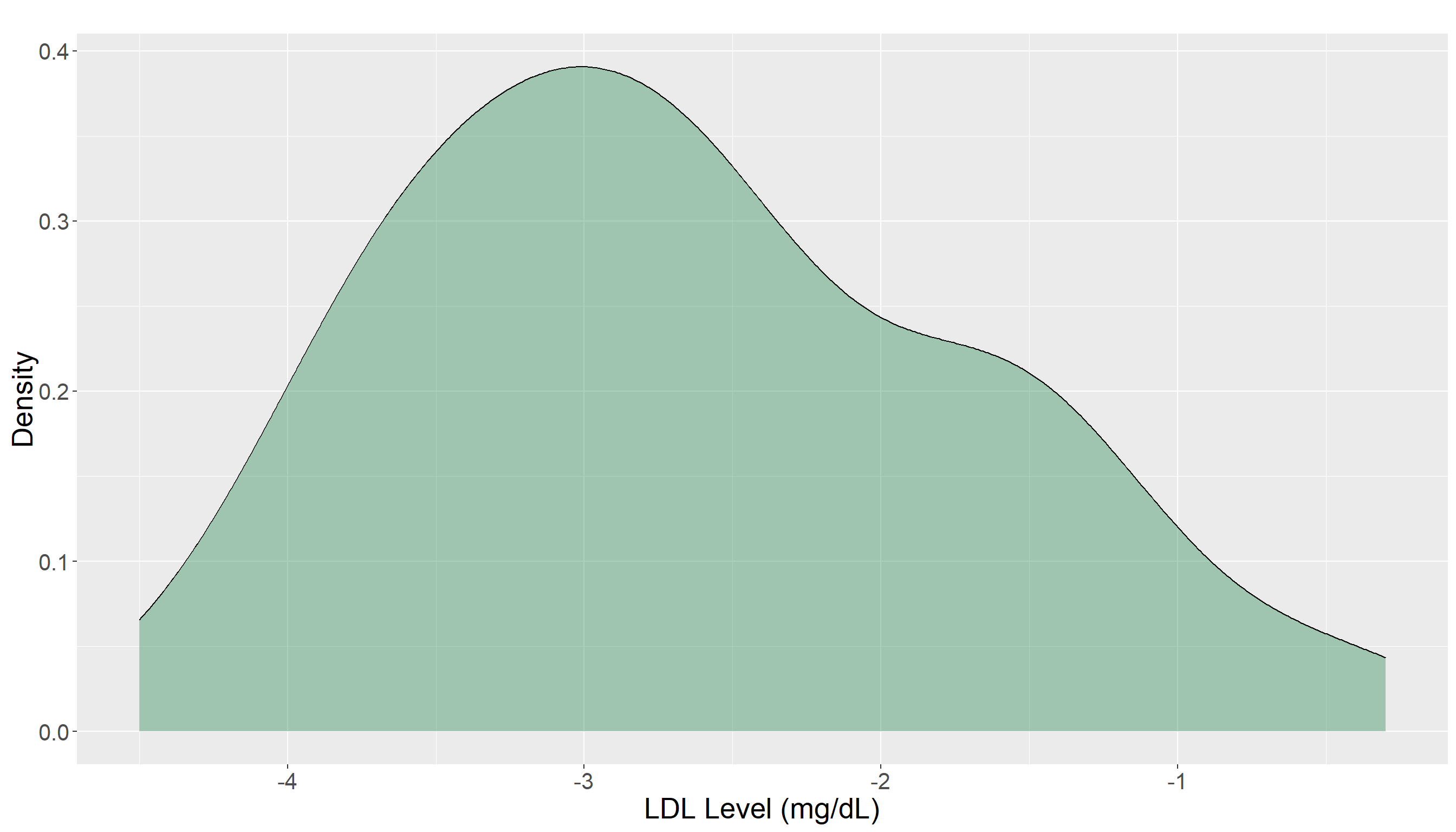
Figure 3.8: Density Plot of Paired LDL Levels Differences

From the density plot, most LDL differences appear to fall below zero with the distribution noticeably centered away from it. This suggests a general decrease in LDL levels after treatment, but the observation should be verified through formal statistical testing. From this plot, it is not clear if this reduction is significant or not.

3.4.5 Testing Settings

We use a significance level of \(\alpha = 0.05\) to conduct the hypothesis test. Since our data represent a sample from a larger population of patients, we define the following population parameter:

\(\mu_{d}\) is the mean difference in LDL levels (after treatment – before treatment) for all patients in the population.

Our goal is to test whether the population mean difference \(\mu_{d}\) is equal to zero. This would indicate no change in LDL levels after treatment versus the alternative that \(\mu_{d}\) is not zero which suggests a treatment effect.

What is \(\mu_s\) as a parameter here?

Here the notation of \(\mu_d\) is the population mean of the differences of \(d_i\) which is an unknown parameter in the population.
To test this hypothesis, we use the paired t-test, which is essentially a one-sample t-test on the differences \(d_1, d_2, \ldots, d_n\).
We test \(\mu_d=0\) because if there is an actual effect of diet on blood pressure, we expect the null hypothesis to be rejected.

3.4.6 Hypothesis Definitions

We now define the null and alternative hypotheses. Recall the main question we posed:

Is the mean LDL level after treatment statistically different from the mean LDL level before treatment for the same patients?

Because the measurements are paired, this question is equivalent to asking whether the mean difference in LDL levels (after - before) is zero. This leads to the following hypotheses:

\[H_0: \mu_d = 0 \quad \textit{(no mean change in LDL levels)}\]

\[H_a: \mu_d \neq 0 \quad \textit{(mean LDL levels change after treatment)}\]

3.4.7 Test Flavour and Components

To test this hypothesis, we use the paired t-test, which compares the mean difference in LDL levels before and after treatment within the same individuals. Note that the test is done on the paired differences. The test accounts for the fact that the measurements are not independent but rather are paired. The test statistic for this test is computed as:

\[t = \frac{\bar{d}}{ s_d / \sqrt{n} } \tag{3.6}\]

where:

\(\bar{d}\) is the mean of the differences in LDL levels (post-treatment minus pre-treatment) for all participants.
\(s_d\) is the standard deviation of these differences and is computed as:

\(s_d = \sqrt{\frac{1}{n-1} \sum_{i=1}^{n} (d_i - \bar{d})^2}\)

\(n\) is the number of paired observations (participants).

3.4.8 Inferential Conclusions

As you can see in Equation 3.6, the statistic divide the sample mean of differences and scale it according to the standard deviation. The idea is very similar to the other tests that we have been working on so far. Under the null hypothesis, the test statistic defined in Equation 3.6 follows a t-distribution with \(n-1\) degrees of freedom. For this test, we can compute the \(\textit{p-value}\) as:

\[\textit{p-value} = 2 \times \Pr(T_{n - 1} \ge |t|)\]

Remember!

When we run this test, we make the following assumptions:

either the sample size is large enough (we are thinking about \(n=30\) at least) so that central limit theorem assumptions work well, or
the distribution of our sample in each group is normal or symmetric enough.

If the normality assumption is also not satisfied (e.g., due to skewed distributions or outliers) or we have a very small sample size, we may turn to a non-parametric alternative, such as the Mann–Whitney–Wilcoxon test, which compares the ranks of the observations across groups rather than the raw values but this book will not cover it. You can read more about it LINK.

3.4.9 How to run the two-sample paired t-test in `R` and `Python`

R Code
Python Code

# Extract LDL measurements before and after treatment
ldl_before <- test_cholesterol |>  pull(LDL_before)
ldl_after  <- test_cholesterol |>  pull(LDL_after)

# Run paired t-test
t.test(x = ldl_before, y = ldl_after, paired = TRUE)


    Paired t-test

data:  ldl_before and ldl_after
t = 18.248, df = 59, p-value < 2.2e-16
alternative hypothesis: true mean difference is not equal to 0
95 percent confidence interval:
 2.141281 2.668719
sample estimates:
mean difference 
          2.405

import pandas as pd
from scipy.stats import ttest_rel

# Load dataset
df = pd.read_csv('data/test_cholesterol.csv')

# Extract LDL measurements before and after treatment
ldl_before = df['LDL_before'].to_numpy()
ldl_after = df['LDL_after'].to_numpy()

# Run paired t-test
t_stat, p_value = ttest_rel(ldl_before, ldl_after)

# Print results
print(f"T-statistic: {t_stat}")

T-statistic: 18.248188665420518

print(f"P-value: {p_value}")

P-value: 6.125701137511457e-26

Details about R code and output

Key arguments of the t.test function in R for a paired test are:

x: numeric vector of measurements before treatment.
y: numeric vector of measurements after treatment.
paired = TRUE: indicates that the samples are related.

The output includes:

statistic: the calculated t-test statistic (here, t = 22.303).
df: the degrees of freedom for t-distribution
p.value: the p-value for testing the null hypothesis that the true mean difference is zero.
conf.int: the 95% confidence interval for the mean difference in LDL levels.
estimate: the estimated mean of the paired differences.

Note: The paired t-test assumes that the differences between pre and post-treatment measurements are approximately normally distributed. Unlike independent sample tests, this test directly accounts for the correlation between repeated measurements on the same patient.

Details about Python code and output

When running a paired t-test in Python using scipy.stats.ttest_rel, the main components are:

x: numeric array of measurements before treatment (ldl_before).
y: numeric array of measurements after treatment (ldl_after).

The output includes:

t_stat: the computed t-test statistic for the paired differences.
p_value: the probability of observing the data if the null hypothesis (no difference) is true.

3.4.10 Storytelling

Based on our analysis, we asked: Did LDL levels change significantly after treatment? The paired t-test gave a very small \(\textit{p-value}\), far below \(\alpha = 0.05\) providing strong evidence against the null hypothesis. In simple terms, this means LDL levels after treatment are significantly lower than before. On average, the reduction was about 2.4 units, with the true effect likely between 2.1 and 2.7 units. In summary, these results indicate that the observed reduction in LDL levels is highly unlikely to have occurred by chance if there were no true effect.

Note: Compare the 2.4-unit reduction that we estimated from our sample to the value we set for the Delta variable in our simulation. Also note that Delta is the true underlying mean reduction built into the simulated population not a value estimated from data. The sample mean reduction (2.4 units) serves as our estimate of this true effect. If our sample is representative and the assumptions of the paired t-test are met, the sample estimate should be close to the true value of Delta as the sample size increases. Also Delta, the true underlying mean reduction, is within boundary estimate of 2.1 and 2.7 units. If you are interested, try running the analysis by increasing the sample size (the n_patients variable in the code) to see what happens to the results!

3.5 Tests for Two Population Proportions

3.5.1 Review

In the examples we studied in Chapter 2, we estimated the proportion of a population based on the sample proportion \(\hat{p}\). This is often the case in practice, as the population proportion is typically unknown and must be inferred from sample data. When we are comparing two groups and wish to test whether their underlying proportions differ, we can extend this idea to a two-proportion test.

Suppose you are investigating support for a new policy among two different regions, Region A and Region B. Each individual either supports the policy (coded as 1) or does not support it (coded as 0). You want to determine if the proportion of supporters of the new policy is significantly different between Region A and Region B.

Formally, let:

Region A (Population 1): each individual either supports the policy (coded as 1) or policy (coded as 0).

Region B (Population 2): defined in the same way.

From each population, we take a random sample:

From Region A, a sample of size \(n\), with observed sample proportion of support \(\hat{p}_A\).
From Region B, a sample of size \(m\), with observed sample proportion of support \(\hat{p}_B\).

where \(\hat{p}_A\) and \(\hat{p}_B\) are the estimates for the \(p_A\) and \(p_B\). Note that \(p_A\) and \(p_B\) are the true proportion of new policy supporters in Region A and Region B and we estimate them by \(\hat{p}_A\) and \(\hat{p}_B\).

The main statistical question becomes: Is there a significant difference between the true population proportions of support in the two regions?

We formalize this as a hypothesis test:

\[ H_0: p_A = p_B \quad \text{versus} \quad H_A: p_A \ne p_B \]

To answer this, we use the two-sample z-test for population proportions, which compares the observed sample proportions (i.e. \(\hat{p}_A\) and \(\hat{p}_B\)) while accounting for the variability expected under the null hypothesis.

3.5.2 Study Design

Consider a survey aimed at estimating support for a new environmental policy in two regions of a country. Researchers randomly sample Region A (n = 150 individuals) and Region B (m = 200 individuals), recording whether each participant supports the new policy. The main outcome of interest is whether an individual supports or does not support the policy. In the next section, we will show the details of a generated dataset to simulate this real scenario in practice.

3.5.3 Data Collection and Wrangling

Similar to previous example, we will work with a simulated dataset that has been specifically created to illustrate the concept of tests for two populations. The code below generates the dataset we will be using. While running these lines is not strictly necessary if you are only interested in following along with the analysis, we recommend reading Appendix B for a deeper understanding of how and why the data were generated in this way.

# Set seed
set.seed(123)

# Set sample sizes
n_A <- 150
n_B <- 200

# Set the values for true population proportions
p_A <- 0.57
p_B <- 0.43

# Generate binary outcomes for survey responses
support_A <- rbinom(n_A, size = 1, prob = p_A)
support_B <- rbinom(n_B, size = 1, prob = p_B)

# Create dataset
policy_data <- data.frame(
  region = c(rep('A', n_A), rep('B', n_B)),
  support = c(support_A, support_B) )

The dataset contains a region column and a support column indicating if the participant supports the policy. To have a better picture of dataset, we take a look at the frequency table.

policy_data |>
  group_by(region) |>
  summarise(count = n()) |>
  arrange( desc(count) )

# A tibble: 2 × 2
  region count
  <chr>  <int>
1 B        200
2 A        150

3.5.4 Exploratory Data Analysis

policy_summary <- policy_data |> 
  group_by(region) |> 
  summarise(n = n(), supporters = sum(support), prop_support = mean(support))
policy_summary

# A tibble: 2 × 4
  region     n supporters prop_support
  <chr>  <int>      <int>        <dbl>
1 A        150         85        0.567
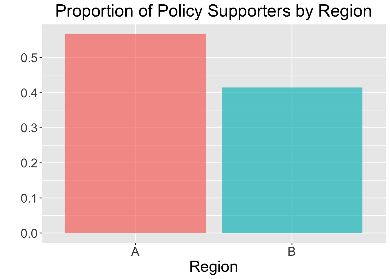
2 B        200         83        0.415

A simple bar plot can also help visualize the differences:

ggplot(policy_summary, aes(x = region, y = prop_support, fill = region)) +
  geom_bar(stat = 'identity', alpha = 0.7) +
  labs(
    x = 'Region', 
    y = '',
    title = 'Proportion of Policy Supporters by Region',
    fill = NULL
  ) +
  scale_y_continuous(breaks = seq(0, 1, by = 0.1)) +
  theme(
    plot.title = element_text(size = 22, hjust = 0.5),
    axis.title.x = element_text(size = 20),
    axis.title.y = element_text(size = 20),
    axis.text = element_text(size = 16),
    legend.text = element_text(size = 16),
    strip.text = element_text(size = 20),
    legend.position = 'none'
  )

3.5.5 Testing Settings

We use a significance level of \(\alpha = 0.05\). The population parameters are:

\(p_A\): true proportion of supporters in Region A.
\(p_B\): true proportion of supporters in Region B.

The goal is to test if the difference \(p_A - p_B\) is significantly different from zero.

3.5.6 Hypothesis Definitions

The null and alternative hypotheses are:

\[H_0:p_A = p_B \quad vs \quad H_1:p_A \neq p_B\]

3.5.7 Test Flavour and Components

The two-sample z-test for proportions is the appropriate method for testing this hypothesis. As with any hypothesis test, we first need to compute the test statistic. For this test, we calculate the pooled proportion as

\[\hat p = \frac{x_A + x_B}{n_A + n_B}\]

where \(x_A\) and \(x_B\) are the counts of successes in the two samples and \(n_A\) and \(n_B\) are the respective sample sizes. The z-statistic is then computed as:

\[z = \frac{\hat p_A - \hat p_B}{ \hat p (1 - \hat p) \left( \frac{1}{n_1} + \frac{1}{n_2} \right)} \tag{3.7}\]

Under \(H_0\), the statistic defined in Equation 3.7 approximately follows a standard normal distribution for large sample sizes. The \(\texttt{p-value}\) is then calculated as:

\[\texttt{p-value} = 2 \times Pr(Z \ge |z|)\]

Standard Normal and Chi-square

The test statistic for comparing two proportions can also be expressed as a chi-squared statistic \(\chi^2\) which under the null hypothesis approximately follows a chi-squared distribution with 1 degree of freedom.
For large sample sizes, it can be shown that this statistic is closely related to the square of the z-statistic (i.e. \(X^2 \approx z^2\)) providing an equivalent measure of the difference between proportions.

3.5.8 Inferential Conclusions

If the \(\textit{p-value}\) is smaller than \(\alpha = 0.05\), we reject \(H_0\), indicating a significant difference in policy support between the two regions. Otherwise, we fail to reject \(H_0\), suggesting no evidence of a difference.

3.5.9 How to run the two-sample paired t-test in `R` and `Python`

R Code
Python Code

# Using policy_summary to get counts and sample sizes
x1 <- policy_summary |>
  filter(region == 'A') |>
  pull(supporters)

x2 <- policy_summary |>
  filter(region == 'B') |>
  pull(supporters)

n1 <- policy_summary |>
  filter(region == 'A') |>
  pull(n)

n2 <- policy_summary |>
  filter(region == 'B') |>
  pull(n)

# Run two-proportion z-test
prop.test(x = c(x1, x2), n = c(n1, n2))


    2-sample test for equality of proportions with continuity correction

data:  c(x1, x2) out of c(n1, n2)
X-squared = 7.3034, df = 1, p-value = 0.006883
alternative hypothesis: two.sided
95 percent confidence interval:
 0.04118315 0.26215018
sample estimates:
   prop 1    prop 2 
0.5666667 0.4150000

The R output contains the following components:

X-squared: The chi-squared test statistic for comparing the two proportions; under the null hypothesis, it approximately follows a chi-squared distribution with 1 degree of freedom - provided a large sample size.
df: Degrees of freedom for the chi-squared statistic (usually 1 for a two-sample test).
p-value: The p-value of the test.
sample estimates: The sample proportions for each group.
95 percent confidence interval: The confidence interval for the difference in proportions.

Note on continuity correction

You notice with continuity correction in the R output of prop.test function. The continuity correction is a small adjustment applied when using a continuous probability distribution (like the normal distribution) to approximate a discrete distribution (like the binomial) in hypothesis testing.
When approximating a discrete distribution, such as the difference in two sample proportions, with a continuous normal distribution, a continuity correction can be applied to improve the approximation. This involves subtracting (or adding) 0.5 in the numerator of the test statistic (scaled appropriately by sample sizes) to account for the fact that the underlying counts are discrete.
The effect of this correction is most noticeable with small sample sizes and becomes negligible as sample sizes increase.
This can be controlled in prop.test function by setting correct = TRUE (default value) to include continuity correction or correct = FALSE to not include this.

import pandas as pd
from statsmodels.stats.proportion import proportions_ztest

# Load dataset
policy_summary = pd.read_csv('data/policy_summary.csv')

# Extract counts and sample sizes
x1 = policy_summary.loc[policy_summary['region'] == 'A', 'supporters'].values[0]
x2 = policy_summary.loc[policy_summary['region'] == 'B', 'supporters'].values[0]

n1 = policy_summary.loc[policy_summary['region'] == 'A', 'n'].values[0]
n2 = policy_summary.loc[policy_summary['region'] == 'B', 'n'].values[0]

count = [x1, x2]
nobs = [n1, n2]

stat, pval = proportions_ztest(count, nobs)

print(f"Z-statistic: {stat:.4f}, p-value: {pval:.4f}")

Z-statistic: 2.8106, p-value: 0.0049

Heads-up!

Note that proportions_ztest function from statsmodels.stats.proportion does NOT provide an argument to control the implementation of continuity correction and by default it doe not make any correction.
As a result the results between R and Python differes. You can write a function in Python to apply this correction and then compute the p-value accordingly but it is not the scope of this textbook.

3.5.10 Storytelling

We surveyed people in two regions to see how much support there is for a new environmental policy. In Region A, a little over half of the participants (57%) were in favor, while in Region B, only about 42% supported it. Statistical testing confirmed that this difference is unlikely to be due to chance: the results suggest that support in Region A is genuinely higher than in Region B with p-value = 0.0068. In fact, we can be reasonably confident that the true difference in support between the regions lies somewhere between 4% and 26%.

3.1 Two sample Student’s t-test for Independent Samples

3.1.1 Review

3.1.2 Study design

3.1.3 Data Collection and Wrangling

3.1.4 Explanatory Data Analysis

3.1.5 Testing Settings

3.1.6 Hypothesis Definitions

3.1.7 Test Flavour and Components

3.1.8 Inferential Conclusions

3.1.9 How to run the test in R and Python?

3.1.10 Storytelling

3.2 Two sample Welch’s t-test for independent samples

3.2.1 Review

3.2.2 Study Design

3.2.3 Data Collection and Wrangling

3.2.4 Explanatory Data Analysis

3.2.5 Testing Settings

3.2.6 Hypothesis Definitions

3.2.7 Test Flavour and Components

3.2.8 Inferential Conclusions

3.2.9 How to run the test in R and Python?

3.2.10 Storytelling

3.3 Two sample z-test for Independent Samples

3.3.1 Review

3.3.2 Study Design

3.3.3 Data Collection and Wrangling

3.3.4 Exploratory Data Analysis

3.3.5 Testing Settings

3.3.6 Hypothesis Definitions

3.3.7 Test Flavour and Components

3.3.8 Inferential Conclusions

3.3.9 How to run the two-sample z-test in R and Python

3.3.10 Storytelling

3.4 Two sample t-test for Paired Samples

3.4.1 Review

3.4.2 Study Design

3.4.3 Data Collection and Wrangling

3.4.4 Exploratory Data Analysis

3.4.5 Testing Settings

3.4.6 Hypothesis Definitions

3.4.7 Test Flavour and Components

3.4.8 Inferential Conclusions

3.4.9 How to run the two-sample paired t-test in R and Python

3.4.10 Storytelling

3.5 Tests for Two Population Proportions

3.5.1 Review

3.5.2 Study Design

3.5.3 Data Collection and Wrangling

3.5.4 Exploratory Data Analysis

3.5.5 Testing Settings

3.5.6 Hypothesis Definitions

3.5.7 Test Flavour and Components

3.5.8 Inferential Conclusions

3.5.9 How to run the two-sample paired t-test in R and Python

3.5.10 Storytelling

3.1.9 How to run the test in `R` and `Python`?

3.2.9 How to run the test in `R` and `Python`?

3.3.9 How to run the two-sample `z-test` in `R` and `Python`

3.4.9 How to run the two-sample paired t-test in `R` and `Python`

3.5.9 How to run the two-sample paired t-test in `R` and `Python`