mindmap
  root((Frequentist
  Hypothesis
  Testings
  ))
    Simulation Based<br/>Tests
    Classical<br/>Tests
      (Chapter 2: <br/>Tests for One<br/>Continuous<br/>Population Mean)
      (Chapter 3: <br/>Tests for Two<br/>Continuous<br/>Population Means)
      (Chapter 4: <br/>ANOVA-related <br/>Tests for<br/>k Continuous<br/>Population Means)
        {{Unbounded<br/>Responses}}
          One<br/>Factor type<br/>Feature
            )One way<br/>ANOVA(
          Two<br/>Factor type<br/>Features
            )Two way<br/>ANOVA(
      (Chapter 5: <br/>Chi-squared<br/>Tests)
4 ANOVA-related Tests for \(k\) Continuous Population Means
Learning Objectives
By the end of this chapter, you will be able to:
- Explain how analysis of variance (ANOVA) partitions total variation into between-group and within-group components.
- Interpret the meaning of the \(F\)-statistic and its role in testing mean differences across groups.
- Describe the difference between main effects and interaction effects in a two-way ANOVA.
- Identify potential interaction patterns via appropriate plotting when conducting a two-way ANOVA.
- Conduct one and two-way ANOVA in a reproducible manner using the hypothesis testing workflow via
RandPython. - Identify the assumptions underlying one-way and two-way ANOVA, including independence, normality, and homoscedasticity.
- Evaluate model diagnostics to assess whether ANOVA assumptions are met.
It is time to expand our hypothesis testing framework from comparing two population means to a generalized approach for \(k\) population means by exploring analysis of variance (ANOVA) as shown in Figure 4.1. ANOVA is a foundational test in frequentist statistics designed to compare means across multiple populations under specific distributional assumptions, which we will examine in this chapter. Originally formalized by Ronald A. Fisher (Fisher 1925), ANOVA extends the concept of the two-sample \(t\)-test by partitioning the total variability of our outcome of interest into components attributable to main effects, interactions, and random error. This partitioning enables us to determine whether observed differences in groups are improbable to appear under the null hypothesis, which states that all groups share the same population mean.
Heads-up on some historical background in statistics!
While Ronald A. Fisher (1890–1962) is rightly recognized as a significant figure in modern statistics for developing key concepts such as ANOVA, it is imperative to recognize the broader context of his legacy. Beyond his pioneering contributions to statistics, Fisher was also a prominent advocate of eugenics, a movement that promoted pseudoscientific ideas about human heredity and social hierarchy. His involvement with the eugenics community is well documented (MacKenzie 1981). These views have been called out by certain members of the scientific community (Tarran 2020). That said, we (the authors of this mini-book) consider that students and scholars need to distinguish Fisher’s statistical insights from the unethical ideologies he supported, while also acknowledging the social responsibility to critique the historical misuse of science.
Fisher’s statistical work remains central to frequentist inference. However, educators and researchers must confront the historical connection between statistical innovation and eugenic thinking in early 20th-century science (Tabery and Sarkar 2015). By explicitly addressing this context, we can acknowledge the rigour of Fisher’s methodological contributions while rejecting the discriminatory worldviews he promoted. This approach aligns with contemporary efforts to ensure that teaching statistics is grounded not only in subject matter accuracy but also in ethical reflection and historical accountability (Kennedy-Shaffer 2024).

The most standard application for ANOVA tests is experimentation. Actually, the origins of ANOVA were in part motivated by agricultural experiments (Fisher 1925). That said, nowadays, ANOVA has significantly expanded in modern inferential applications, and it has contributed substantially to the advancement in modern data science. The examples in this chapter are written in the spirit of online controlled experiments (i.e., a style of randomized experimentation that is used in product and marketing analytics).
Heads-up on the importance of ANOVA in data science!
In modern data science, ANOVA remains significant, particularly in A/B/n testing (the generalization of A/B testing to multiple treatments). This approach allows for the simultaneous evaluation of various treatment variations or designs. ANOVA is valued for its interpretability and its flexibility in handling both balanced designs (where there is an equal number of replicates for each experimental treatment) and unbalanced designs (where there are unequal numbers of replicates). These strengths have solidified its role in both academic research and practical applications.

In practice, work teams rarely test only one new experimental idea at a time. Hence, it is common to ship multiple variants in the same experiment such as: three checkout layouts, four headline options or five recommendation-ranking tweaks. This generalization is what A/B/n testing is, where n simply means “more than two variants.” The moment we move from two to many variants, a tempting (but risky!) strategy is to run many pairwise \(t\)-tests. The risk is multiplicity: the more tests we run, the more likely we are to see a “significant” result somewhere purely by chance (i.e., we are more prone to commit Type I errors!). That said, ANOVA provides a clean first step: it gives an overall test of whether any mean differs, using a single test statistic and a single \(p\)-value.
Heads-up on ANOVA as a primary overall test!
In many experiments, ANOVA is best understood as a two-part process:
-
Overall test. We test whether the group means are all equal (i.e., we run one \(F\)-test as explained further in this chapter).
- Follow-up test. Only if warranted, we must investigate which means differ using a multiple-comparisons procedure that controls the overall error rate (e.g., Tukey’s HSD).
This two-step process is a safe way to avoid over-interpreting random noise at first when many different experimental variants are on the table.
The simulated datasets discussed in this chapter relate to the aforementioned experimental context called A/B/n testing, which is a generalization of the traditional A/B testing as previously discussed. In a typical A/B testing, participants are randomly assigned to one of two strategies, referred to as treatments: treatment \(A\) (the control treatment) and treatment \(B\) (the experimental treatment). This approach enables us to infer causation concerning the following inquiry:
Will changing from treatment \(A\) to treatment \(B\) cause my outcome of interest, \(Y\), to increase (or decrease, if that is the case)?

Note that, in an ANOVA setting, the outcome must be continuous. Furthermore, the primary goal of A/B testing is to determine whether there is a statistically significant difference between treatments \(A\) and \(B\) concerning the outcome. It is important to stress that, because we are dealing with randomized experiments which allows us to get rid of the effect of further confounders, we can talk about causal effects (not just associations), provided random assignment is implemented properly and the experimental protocol is respected. This is why our upcoming main inferential inquiries will be phrased in causal language (e.g., “does changing the design cause the mean score to change?”) rather than purely association phrasing.
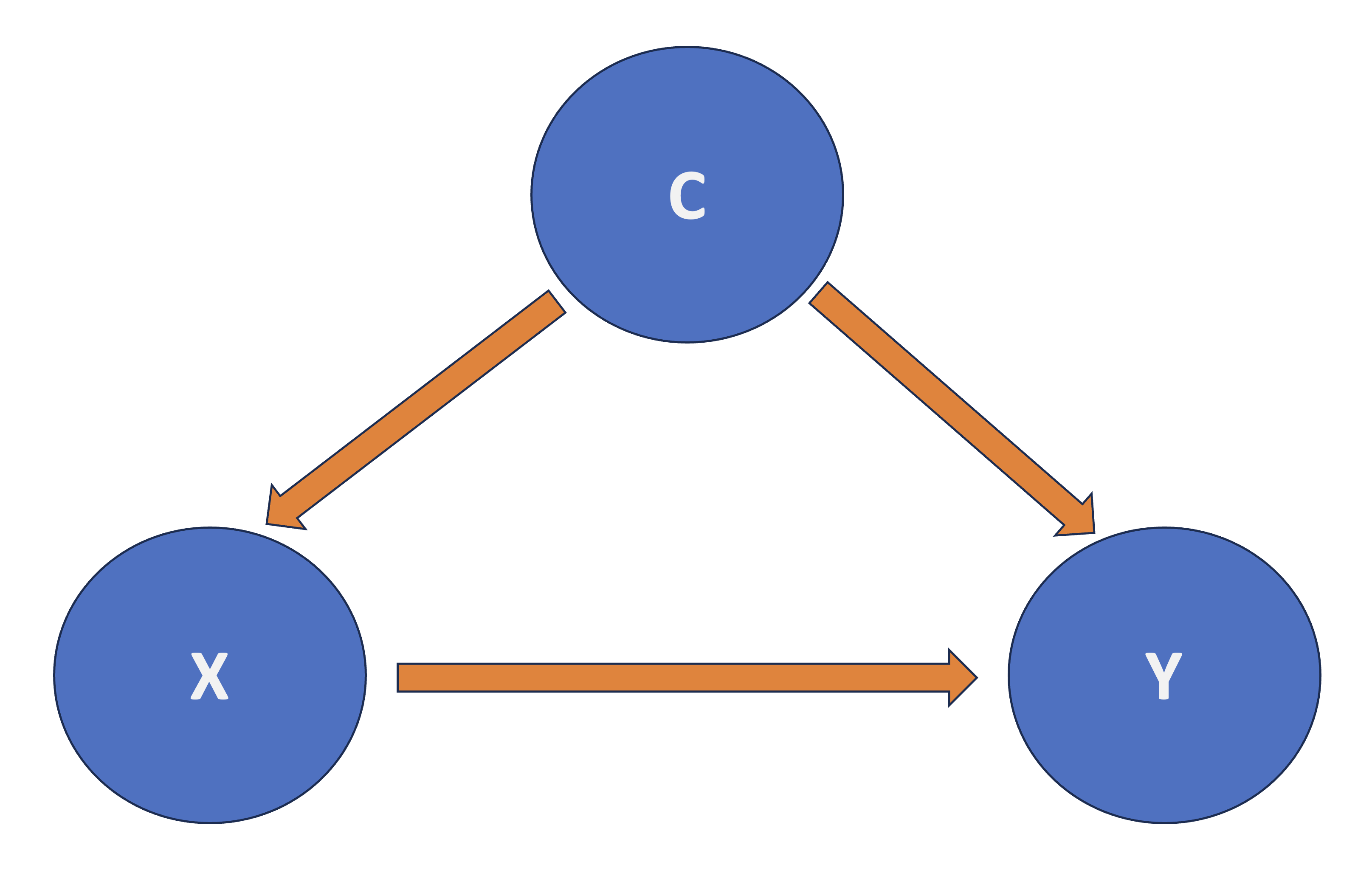
Heads-up on confounding!
In causal inference, confounding refers to the mixing of effects between the outcome of interest, denoted as \(Y\), the randomized factor \(X\) (which is a two-level factor in A/B testing, corresponding to treatment \(A\) and treatment \(B\)), and a third, uncontrollable factor known as the confounder \(C\). This confounder is associated with the factor \(X\) and independently affects the outcome \(Y\), as shown by Figure 4.2.
With that framing in mind, we can now proceed with our two ANOVA cases (one-way and two-way) and their corresponding datasets to illustrate how this statistical approach can be applied via the structured test workflow from Figure 1.1 found in Section 1.1. As a side note, this chapter builds on the concepts introduced in the earlier works by Chapter 2 and Chapter 3, which concentrated on hypothesis testing for one and two groups, respectively. While those chapters primarily addressed pairwise comparisons, we will now shift our focus to multiple comparisons:
- The one-way ANOVA, discussed in Section 4.1, will assume a single categorical factor with \(k\) levels. This approach allows us to test whether at least one group mean is significantly different from the others.
- In contrast, the two-way ANOVA, from Section 4.2, will incorporate an additional categorical factor with \(m\) levels, permitting the analysis of both main effects and interaction effects. Interaction terms in ANOVA are especially useful for revealing cases where the effect of one factor depends on the level of another, a situation often encountered in complex experimental designs.
Tip on a further A/B testing resource!
If you would like to check an industry-focused guide to A/B testing pitfalls, you can check the book by Kohavi, Tang, and Xu (2020).

4.1 One-way ANOVA
Imagine you are a data scientist at well-known food delivery app working with a cross-functional “Growth” team (product, marketing, and engineering). The company is heavily invested in statistical experimentation on its app to enhance the customer experience, aiming to increase long-term profit margins. As part of this effort, the team frequently conducts A/B/n testings on the checkout funnel. These A/B/n testings have a clear business goal:
We must increase the average customer conversion score.
For this chapter, in general, we treat the conversion score as a continuous and unitless index (whose baseline is around \(50\)) that rolls up three signals: completed orders, checkout completion speed, and meaningful engagement. Higher scores mean customers are moving through the funnel more successfully. Having said all this, to start with the first of the two A/B/n testings in this chapter, let us suppose the stakeholders have come up with the groundbreaking idea of modifying the checkout-page design in two different experimental ways to investigate whether these modifications somehow cause the average customer conversion score to change. For the sake of this one-way ANOVA case, the designs are the following:
-
\(D_1\): the current (control) design,
-
\(D_2\): a new design that simplifies the checkout layout,
- \(D_3\): a new design that highlights delivery-time estimates earlier.
This is exactly the kind of “more than two variants” experiment where one-way ANOVA becomes the natural inferential tool.

4.1.1 Study Design
The first stage of our testing workflow involves the main statistical inquiry we aim to address. Therefore, let us translate the above situation into a concrete question that is meaningful for both the stakeholders and for you as part of the this “Growth” team. We can frame the main inquiry as follows:
Does changing the checkout page design (from \(D_1\) to \(D_2\) or \(D_3\)) cause a difference in the population mean conversion score?

This statistical inquiry represents the foundational step in our testing workflow. We transform a practical business question into a testable inferential statement (specifically, a causal one). By framing the problem as whether the average customer conversion score varies across different checkout-page designs, we connect stakeholder demands with statistical analysis.
In terms on how this A/B/n testing would be designed, let us consider the following aspects:
- The experiment will solely focus on checkout-page design, which we consider a controllable factor determined by the experimenter (that is you, as part of the work team). This factor includes three different checkout-page layouts (or designs): \(D_1\) (the current layout), \(D_2\) (a new and experimental layout), and \(D_3\) (another new and experimental layout). This setup creates a three-level factor. To summarize in statistical terms, we have:
- One factor: checkout design.
- Three treatments (the three layout options), which classifies this study as A/B/n testing. Treatment \(D_1\) is referred to as the control treatment, whereas \(D_2\) and \(D_3\) are the experimental treatments.
- The continuous outcome variable \(Y\), defined as the customer conversion score, which has been explained previously.
- Before conducting the experiment, assume that your team has performed a proper power analysis (with a significance level \(\alpha = 0.05\) and power \(1 - \beta = 0.8\)) to determine the total sample size of customers to be recruited for the A/B/n testing so you can detect a large enough effect size. This power analysis has indicated an overall sample size of \(n = 600\) customers (namely, experimental units) . Consequently, each treatment group will consist of \(\frac{n}{3} = 200\) customers, making this a balanced experiment.
Heads-up on the importance of having a balanced experiment!
In the design and analysis of experiments, having a balanced experiment (where each treatment receives the same number of experimental units) offers two advantages:
- Statistically, a balanced experiment helps minimize the uncertainty in estimating the population parameters necessary for hypothesis testing, which is essential for addressing our main statistical inquiries.
- On the other hand, from a practical point of view, a balanced experiment makes analysis robust against biased parameter estimation, which might be caused by an uneven exposure of experimental units to the different treatments.

4.1.2 Data Collection and Wrangling
Having designed our statistical experiment, it is now time to execute it, which we refer to as data collection. To ensure we accurately assess the causality of our statistical inquiry regarding changes in the population mean customer conversion score across three different checkout designs, we must randomly assign our \(n = 600\) experimental units evenly among the three treatments. This means we will collect \(\frac{n}{3} = 200\) data points for each treatment. To achieve this, we can use a suitable online tool to route website traffic uniformly, potentially employing stratified randomization based on additional covariates, such as device type and geographical location. This approach will help us allocate the \(n = 600\) experimental units to one of the three treatments effectively.
Heads-up on the importance of treatment randomization in statistical experimentation!
In A/B and A/B/n testing, online tools such as Optimizely and ABTasty enable experimenters to randomly assign web traffic units (i.e., experimental units) to different treatments of interest. These tools also offer several additional useful features, which are beyond the scope of this textbook.
Treatment randomization is a valuable statistical tool because:
- It ensures that, on average, observed and unobserved confounding variables are evenly distributed across treatments. This helps to avoid obtaining biased estimates of population parameters when evaluating causality between outcomes and the treatments of interest.
- As discussed further in Section 4.1.6, treatment randomization also guarantees that all observed data points are statistically independent concerning the random noise associated with their corresponding measurements. This statistical independence in the random noise (often referred to as the random component, which is also assumed to be identically distributed) is a critical assumption in ANOVA hypothesis testing. If these probabilistic assumptions are not met, the ANOVA test statistic and null distribution may not be appropriate for our observed data and inferential inquiries.

Let us discuss our data collection process. Assume you have already conducted this A/B/n testing and recruited \(n = 600\) customers for this experiment. These customers have been randomly assigned to one of the three checkout designs, and their conversion scores have been measured accordingly. To begin our inferential process, the following code snippets in R and Python (where the library {pandas} is used) will load the dataset, which contains the following columns:
-
checkout_design: A categorical-type column representing the checkout design to which each experimental unit was assigned (\(D_1\), \(D_2\) or \(D_3\)). -
conversion_score: A numeric, continuous column that records the measured customer conversion scores as previously described at the beginning of this one-way ANOVA section.
# Importing library
import pandas as pd

# Loading dataset
OneWay_ABn_customer_data = pd.read_csv("data/ABn_customer_data_one_factor.csv")

# Showing the first 100 customers of the A/B/n testing
print(OneWay_ABn_customer_data.head(100))Tip on the generative modelling process for the simulated data!
We have already clarified that the datasets used in this chapter, such as OneWay_ABn_customer_data, are simulated. We chose this approach to explain ANOVA so that the data used in our test workflow meets the modelling assumptions. This ensures that we can provide a clear and comprehensive explanation for the reader on this inferential tool.
If you are interested in the generative modelling process for OneWay_ABn_customer_data and would like to reproduce it in either R or Python, you can refer to Section B.3.1. Note that the datasets used in this chapter are generated using R, as R and Python use different pseudo-random number generators, even when using the same seeds, leading to different simulated datasets.
Now, after collecting the data, it is time to proceed with the data splitting into training and testing. For this specific case, assume the team in charge of this analysis decided to execute a 50-50 random data splitting which would yield a training set size of \(n_{\text{training}} = 300\) and testing set size of \(n_{\text{testing}} = 300\). Nevertheless, to keep the balanced nature of our experiment, we have to ensure that both sets will end up with 100 customers allocated to each one of the three treatments. Therefore, we need to implement a stratified randomization (where each treatment is a strata) as follows:
-
R: The code in Listing 4.1 performs a stratified random split of theOneWay_ABn_customer_datadataset into training and testing sets, ensuring reproducibility and balance across different levels ofcheckout_design. The library {rsample} (Frick et al. 2025) is utilized for executing the stratified random split. Note that theset.seed()function is used to fix the random seed, allowing the results to be replicated. Then, theinitial_split()function divides theOneWay_ABn_customer_datainto two parts, allocating 50% for training and 50% for testing while maintaining proportional representation of each category in thecheckout_designvariable (thestrataargument ensures this). Thetraining()andtesting()functions extract the respective subsets from the split object. Lastly, to implement a sanity check, we retrieve the dimensions of each subset (number of rows and columns) and examine the relative proportions ofcheckout_designlevels within each split. This sanity check ensures that the experimental treatments remain balanced in both training and testing sets, which is essential for unbiased modelling and valid inference in classical one-way ANOVA.

-
Python: The code in Listing 4.2 executes a stratified data splitting process similar to itsRequivalent, utilizing thetrain_test_split()function from {scikit-learn} (Pedregosa et al. 2011). A fixed random seed is set using therandom_stateparameter to ensure reproducibility, so that each execution generates the same random partition. The dataset,OneWay_ABn_customer_data, is then divided into two equal subsets: 50% for training and 50% for testing. Thestratifyargument intrain_test_split()guarantees that thecheckout_designmaintains consistent proportional representation in both subsets, thus preserving balance across experimental treatments. After completing the split, we conduct the same sanity check as described above.
# Loading library
library(rsample)

# Seed for reproducibility
set.seed(123)

# Randomly splitting into training and testing sets by checkout_design
OneWay_ABn_customer_data_splitting <- initial_split(OneWay_ABn_customer_data,
  prop = 0.5, strata = checkout_design
)

# Assigning data points to training and testing sets
OneWay_ABn_training <- training(OneWay_ABn_customer_data_splitting)
OneWay_ABn_testing <- testing(OneWay_ABn_customer_data_splitting)

# Sanity check
cat(sprintf(
  "Training shape: %d %d\nTesting shape:  %d %d\n\n
Training proportions (checkout_design):\n%s\n\nTesting proportions (checkout_design):\n%s\n",
  nrow(OneWay_ABn_training), ncol(OneWay_ABn_training),
  nrow(OneWay_ABn_testing), ncol(OneWay_ABn_testing),
  paste(capture.output(prop.table(table(OneWay_ABn_training$checkout_design))),
    collapse = "\n"
  ),
  paste(capture.output(prop.table(table(OneWay_ABn_testing$checkout_design))),
    collapse = "\n"
  )
))
Training shape: 300 2
Testing shape: 300 2
Training proportions (checkout_design):
D1 D2 D3
0.3333333 0.3333333 0.3333333
Testing proportions (checkout_design):
D1 D2 D3
0.3333333 0.3333333 0.3333333 # Importing function
from sklearn.model_selection import train_test_split
# Seed for reproducibility
random_state = 123
# Randomly splitting into training and testing sets by checkout_design
OneWay_ABn_training, OneWay_ABn_testing = train_test_split(
OneWay_ABn_customer_data,
test_size=0.5,
stratify=OneWay_ABn_customer_data["checkout_design"],
random_state=random_state
)
# Sanity check
print(
f"Training shape: {OneWay_ABn_training.shape}\n"
f"Testing shape: {OneWay_ABn_testing.shape}\n"
f"\nTraining proportions:\n{OneWay_ABn_training['checkout_design'].value_counts(normalize=True)}"
f"\n\nTesting proportions:\n{OneWay_ABn_testing['checkout_design'].value_counts(normalize=True)}"
)Training shape: (300, 2)
Testing shape: (300, 2)
Training proportions:
checkout_design
D2 0.333333
D3 0.333333
D1 0.333333
Name: proportion, dtype: float64
Testing proportions:
checkout_design
D1 0.333333
D3 0.333333
D2 0.333333
Name: proportion, dtype: float644.1.3 Exploratory Data Analysis
Using our OneWay_ABn_training dataset, which consists of \(n_{\text{training}} = 300\) experimental units, we will carry out a exploratory data analysis (EDA) to provide descriptive insights for our stakeholders. These insights will be delivered alongside inferential conclusions at the end of this workflow. Before we explore the relevant plots for the outcome and treatments used in this experiment, let us first examine some useful summary statistics.
Both Listing 4.3 and Listing 4.4 (in R and Python, respectively) take the data frame OneWay_ABn_training and compute descriptive summaries of the continuous outcome variable conversion_score, grouped by the categorical variable checkout_design. The computations include three basic summary measures:
- the mean conversion score (i.e., average performance of each checkout design),
- the standard deviation (i.e., the within-group variability in customer conversion behaviour), and
- the sample size
n(i.e., number of observations per treatment or checkout design).
These summaries provide a quick and exploratory understanding of the data, helping us obtain descriptive insights into the central tendency and spread of our outcome of interest per experimental treatment. The R implementation in Listing 4.3 uses the {tidyverse} meta-package. Conversely, the Python implementation in Listing 4.4 uses the {pandas} library for these numerical computations.
Heads-up on the use of {reticulate} in the Python code snippet!
In the below Listing 4.4 in Python, we are importing the OneWay_ABn_training set (from Listing 4.1), which was created from our random data splitting in the R environment via the {reticulate} package (Ushey, Allaire, and Tang 2025). We will eventually also do the same with the OneWay_ABn_testing dataset. This approach is necessary because both the {rsample} package in R (used in Listing 4.1) and {scikit-learn} in Python (used in Listing 4.2) utilize different pseudo-random number generators. As a result, they produce different training and testing data splits, even when using the same seed values. Therefore, to ensure consistent output across all subsequent R and Python snippets in our workflow, it is necessary that we use the same training and testing sets.
# Loading library
library(tidyverse)
# To import R-generated datasets to Python environment
library(reticulate)

# Computing summaries
OneWay_summary_table <- OneWay_ABn_training |>
  group_by(checkout_design) |>
  summarise(
    mean_conversion = round(mean(conversion_score), 2),
    sd_conversion = round(sd(conversion_score), 2),
    n = n()
  ) |>
  arrange(checkout_design)
OneWay_summary_table
# A tibble: 3 × 4
checkout_design mean_conversion sd_conversion n
<chr> <dbl> <dbl> <int>
1 D1 60.1 2.9 100
2 D2 60.4 3.05 100
3 D3 60.3 3.05 100# Importing library
import numpy as np
# Importing R-generated training set via R library reticulate
OneWay_ABn_training = r.OneWay_ABn_training
OneWay_summary_table = (
OneWay_ABn_training
.groupby("checkout_design")
.agg(
mean_conversion=("conversion_score", lambda x: round(np.mean(x), 2)),
sd_conversion=("conversion_score", lambda x: round(np.std(x, ddof=1), 2)),
n=("conversion_score", "count")
)
.reset_index()
.sort_values("checkout_design")
)
OneWay_summary_table| checkout_design | mean_conversion | sd_conversion | n | |
|---|---|---|---|---|
| 0 | D1 | 60.11 | 2.90 | 100 |
| 1 | D2 | 60.35 | 3.05 | 100 |
| 2 | D3 | 60.28 | 3.05 | 100 |
The sample average conversion scores (found in the outputs from Listing 4.3 and Listing 4.4) are very similar across the three checkout designs, ranging narrowly from 60.11 to 60.35. Additionally, the sample standard deviations are also alike, with values ranging from 2.9 to 3.05. These standard deviations suggest similar levels of variability within each design. Although there are minor differences in the treatment means, they are subtle enough that formal hypothesis testing, such as one-way ANOVA, is necessary to determine whether these small fluctuations are due to random variation or represent genuine differences in the population means. These summary statistics therefore provide a solid descriptive check on group comparability and the plausibility of ANOVA assumptions, which sets the stage for a rigorous subsequent inferential analysis.
We will use two plots in our EDA: three side-by-side histograms (one per treatment) to compare the continuous conversion scores and three side-by-side boxplots of these scores per treatment. We use R’s {ggplot2}, from {tidyverse}, along with Python’s {matplotlib} and {seaborn}. The side-by-side histograms in Figure 4.3 or Figure 4.4 indicate the following:
- The three checkout designs exhibit approximately unimodal and roughly symmetric distributions centred around conversion scores in the low-60s, with slight differences in spread.
- Design \(D_1\) appears slightly more concentrated around its sample average, while \(D_2\) and \(D_3\) show marginally wider dispersion, reflected in slightly flatter histogram peaks.
- The distributions and central tendencies (i.e., average conversion scores) are pretty similar across the three checkout designs.
hist_one_way <- ggplot(
  OneWay_ABn_training,
  aes(x = conversion_score, fill = checkout_design)
) +
  geom_histogram(
    alpha = 0.7,
    bins = 30,
    color = "white"
  ) +
  labs(
    x = "Conversion Score",
    y = "Count",
    fill = "Webpage Design"
  ) +
  theme_bw(base_size = 14) +
  theme(
    axis.text = element_text(size = 15.5),
    axis.title.x = element_text(size = 20),
    axis.title.y = element_text(size = 20, vjust = 0.5),
    strip.text = element_text(size = 20),
    legend.position = "none"
  ) +
  facet_wrap(~ checkout_design, nrow = 1) +   # <-- horizontal panels
  scale_fill_manual(
    values = c(
      "D1" = "#E69F00",
      "D2" = "#56B4E9",
      "D3" = "#009E73"
    )
  )

hist_one_way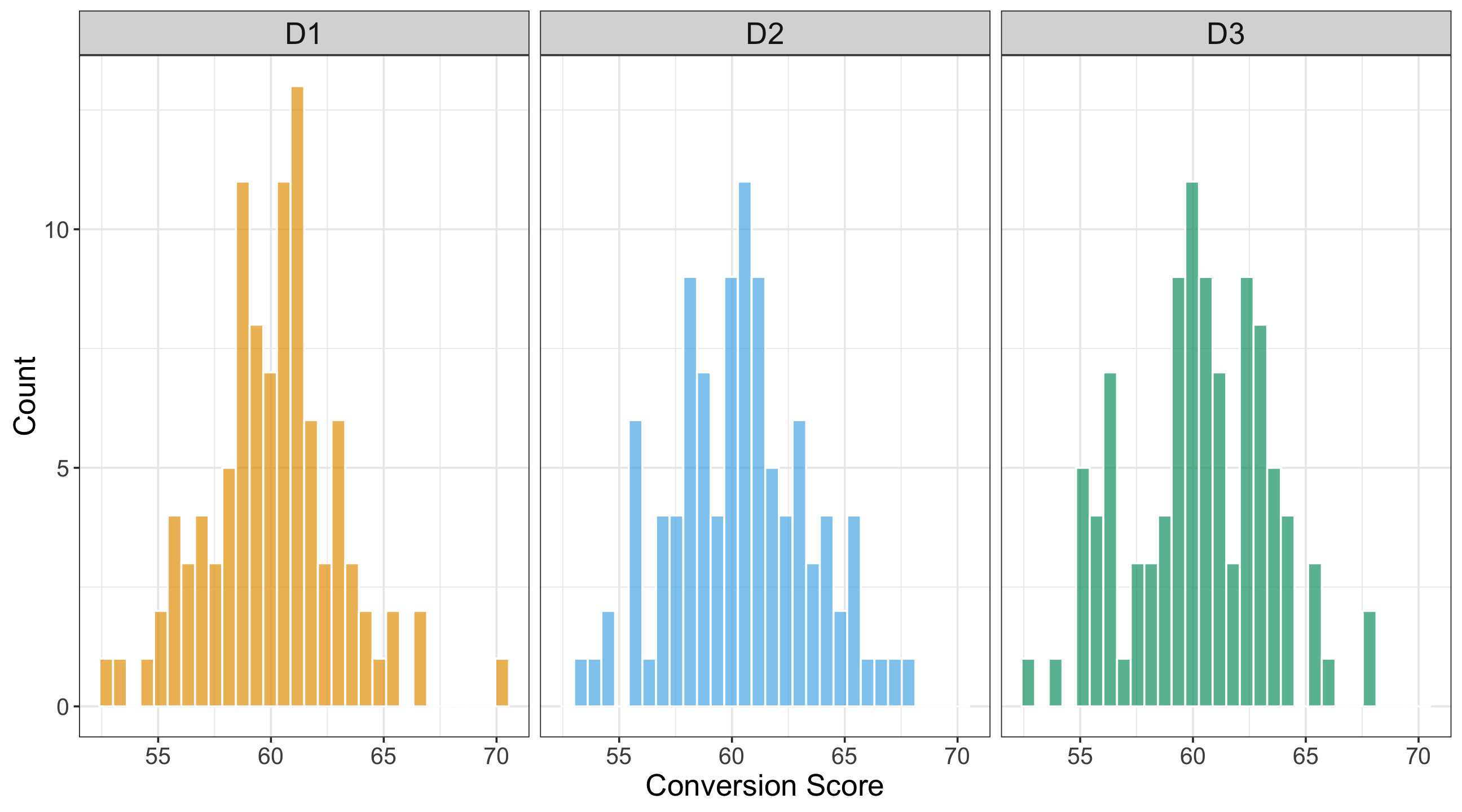
# Importing libraries
import matplotlib.pyplot as plt
import seaborn as sns

# Setting white-grid theme and typography
sns.set_theme(style="whitegrid")
plt.rcParams.update({
    "axes.labelsize": 20,
    "axes.titlesize": 20,
    "xtick.labelsize": 15.5,
    "ytick.labelsize": 15.5,
})

# Defining palette
palette = {
    "D1": "#E69F00",
    "D2": "#56B4E9",
    "D3": "#009E73"
}

design_order = ["D1", "D2", "D3"]

# Creating 1x3 panel layout
fig, axes = plt.subplots(
    1, 3,
    sharex=True,
    sharey=True,
    figsize=(13.5, 7.5)
)

for ax, design in zip(axes, design_order):
    subset = OneWay_ABn_training[
        OneWay_ABn_training["checkout_design"] == design
    ]

    sns.histplot(
        data=subset,
        x="conversion_score",
        bins=30,
        edgecolor="white",
        alpha=0.7,
        color=palette[design],
        ax=ax
    )

    ax.set_title(design, fontsize=20)
    ax.set_xlabel("Conversion Score")

    if ax is axes[0]:
        ax.set_ylabel("Count")
    else:
        ax.set_ylabel("")

# Cleaning up spines and layout
sns.despine(fig=fig)
fig.tight_layout()

plt.show()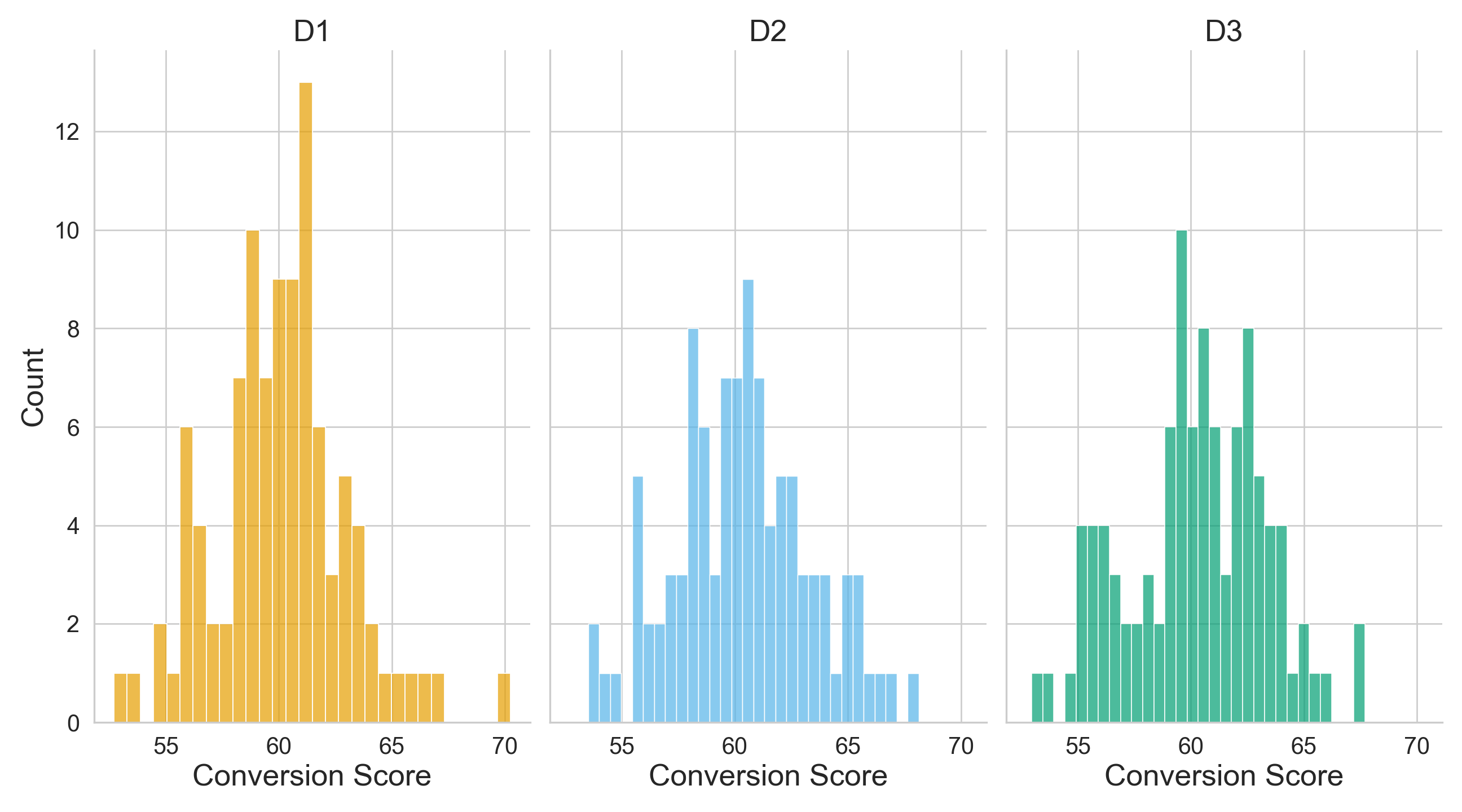
Now, in Figure 4.5 or Figure 4.6, each boxplot represents the distribution of customer conversion scores for one of the three checkout designs (\(D_1\), \(D_2\), and \(D_3\)). The central line in each box is the sample median score; the top and bottom of the box span the 25th to 75th percentiles (the interquartile range, IQR); and the whiskers extend to the non-outlier extremes (according to the conventional 1.5× IQR rule). From a visual comparison of the three treatments (i.e., designs), we have the following:
- The sample medians of \(D_1\), \(D_2\), and \(D_3\) appear quite similar, indicating that the central tendency of conversion score is roughly equivalent across the three checkout designs.
- The box heights (i.e., IQRs) show that the spread of the middle 50% of scores is also very similar across experimental treatments, meaning no checkout design shows substantially more variability in the core of its distribution than the others.
- The whiskers and any outlier points (dots beyond whiskers) may reveal slight differences. For example, if one design has a somewhat longer upper whisker, that signals a larger tail of higher conversion scores in that design.
boxplots_checkout_design_one_way <- ggplot(OneWay_ABn_training, aes(
  x = checkout_design, y = conversion_score,
  fill = checkout_design
)) +
  geom_boxplot(alpha = 0.7, outlier.color = "black") +
  labs(
    x = "Checkout Design",
    y = "Conversion Score"
  ) +
  theme_minimal(base_size = 14) +
  theme_bw() +
  theme(
    axis.text = element_text(size = 15.5),
    axis.title.x = element_text(size = 20),
    axis.title.y = element_text(size = 20, vjust = 0.5),
    strip.text = element_text(size = 20)
  ) +
  theme(legend.position = "none") +
  scale_fill_manual(values = c("D1" = "#E69F00", "D2" = "#56B4E9", "D3" = "#009E73"))
boxplots_checkout_design_one_way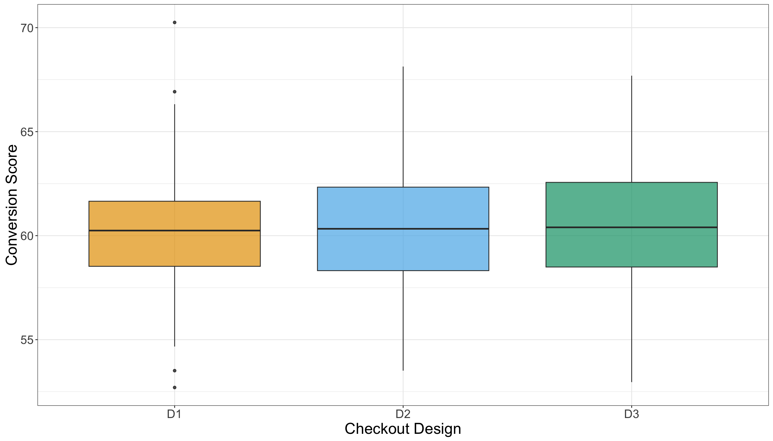
# Setting white-grid theme and typography
sns.set_theme(style="whitegrid")
plt.rcParams.update({
    "axes.labelsize": 20,
    "axes.titlesize": 20,
    "xtick.labelsize": 15.5,
    "ytick.labelsize": 15.5
})

# Defining palette
palette = {
    "D1": "#E69F00",
    "D2": "#56B4E9",
    "D3": "#009E73"
}

# Creating figure
fig, ax = plt.subplots(figsize=(14, 8))

# Side-by-side boxplots
sns.boxplot(
    data=OneWay_ABn_training,
    x="checkout_design",
    y="conversion_score",
    palette=palette,
    saturation=0.7,
    linewidth=1.2,
    fliersize=4,
    boxprops={"alpha": 0.7},
    ax=ax
)

# Axis labels and formatting
ax.set_xlabel("Checkout Design", fontsize=20)
ax.set_ylabel("Conversion Score", fontsize=20)

# Removing legend
ax.legend_.remove() if ax.get_legend() else None

# Setting background
sns.despine(offset=10, trim=True)
fig.tight_layout()

# Displaying
plt.show()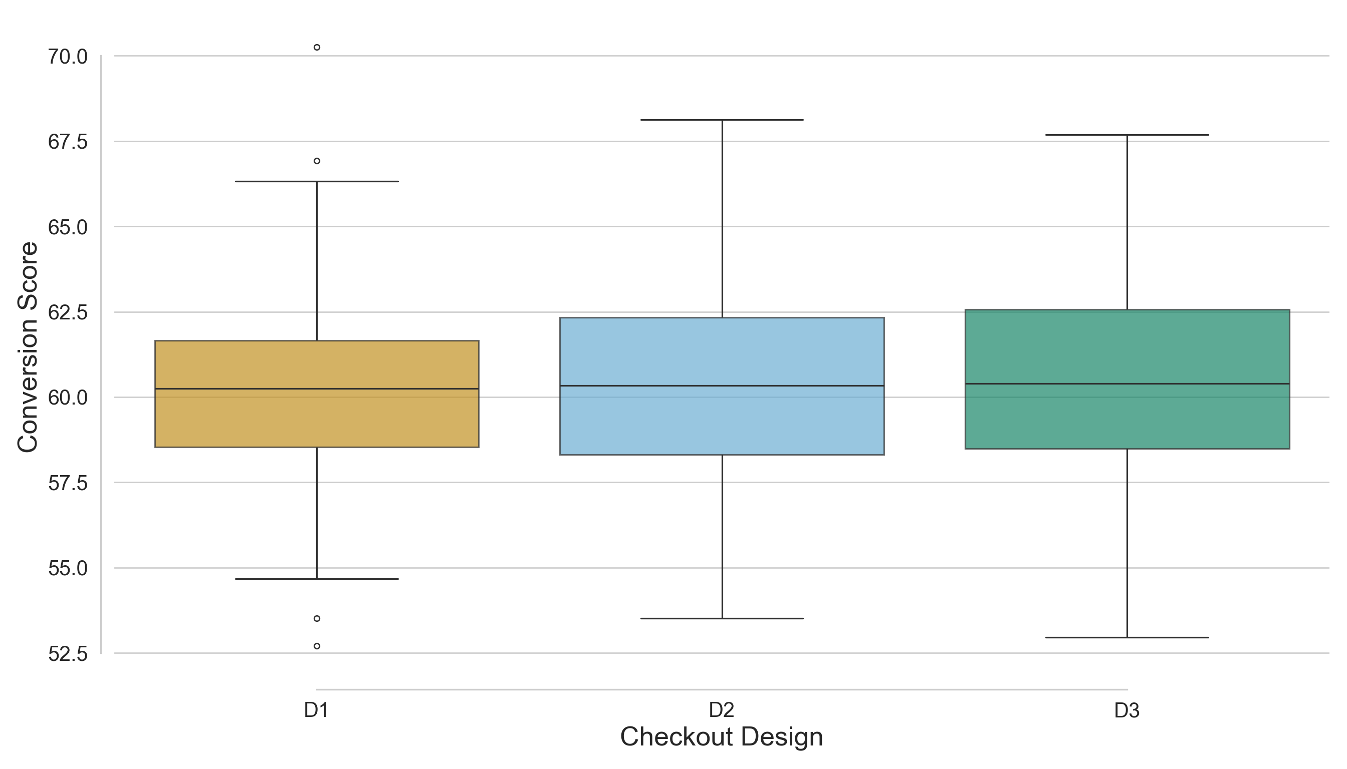
The side-by-side histograms and boxplots indicate that there is no strong visual separation among the distributions of customer conversion scores for the three checkout designs. The central tendency, spread, and tails of the distributions overlap significantly, suggesting that any treatment effect (if it exists) is likely to be subtle rather than pronounced. In summary, the EDA evidence reveals only minor differences among the checkout designs, highlighting the need for formal statistical testing to determine whether these small observed variations are statistically significant or merely a result of random sampling variability.
4.1.4 Testing Settings
Now, let us move to the one-way ANOVA settings before outlining our corresponding hypotheses. Via our training data, the EDA results in Section 4.1.3 suggest a very clear graphical fact: the three checkout designs look quite similar in regards to descriptive statistics and distributional plots, and any possible treatment effect appears subtle. The sample average conversion scores reported in Listing 4.3 (or Listing 4.4) are very similar across treatments \(D_1\), \(D_2\), and \(D_3\), ranging narrowly from 60.11 to 60.35, and the corresponding sample standard deviations are also alike, ranging from 2.9 to 3.05. Visually, the side-by-side histograms in Figure 4.3 (or Figure 4.4) show approximately unimodal, roughly symmetric distributions centred in the low-60s, while the side-by-side boxplots in Figure 4.5 (or Figure 4.6) show sample medians and IQRs that are quite similar across the three designs. Taken together, these descriptive findings support two key takeaways we want to carry over in our testing workflow:
- Any difference in population means (if it exists!) might not be statistically significant, and
- the overall similarity in spreads would make an equal-population-variance assumption reasonable across the three treatments (while still requiring formal diagnostics later).

Having all the above EDA context in mind, we can proceed to the frequentist testing settings used to evaluate whether the small observed differences in conversion scores across the three treatments are beyond random fluctuation. Each population parameter used in our one-way ANOVA must be defined to match the stakeholder question about deployment:
- \(\mu_{D_1}\) is the fixed population mean conversion score we would expect if all eligible customers were shown design \(D_1\) (i.e., the control treatement) under our A/B/n protocol.
- \(\mu_{D_2}\) is the analogous fixed population mean conversion score if all eligible customers were instead shown design \(D_2\) (i.e., the first experimental treatement) under our A/B/n protocol.
- \(\mu_{D_3}\) is the other analogous fixed population mean conversion score under design \(D_3\) (i.e., the second experimental treatement).
\(\mu_{D_1}\), \(\mu_{D_2}\), and \(\mu_{D_2}\) are the corresponding population means (or averages, if we adapt the statistical terminology to the stakeholders’ context) under hypothetical experimental rollouts, and that is exactly why they are the parameters of interest for the “Growth” team:
A decision like “ship experimental checkout design \(D_2\) (or \(D_3\), if that is the case) to production” is ultimately a claim about what would happen on average in the customer population if \(D_2\) (or \(D_3\)) were deployed.
Heads-up on sample versus population language!
In this chapter, we avoid phrasing like “the sample mean under \(D_2\) is higher than the sample mean under \(D_1\)” when making inferential claims, because ANOVA is not about describing our dataset. It is about learning (with uncertainty via sampled data coming from the A/B/n testing) about population quantities that stakeholders care about such as \(\mu_{D_1}\), \(\mu_{D_2}\), and \(\mu_{D_3}\).

The observed group averages \(\bar{y}_{D_1}\), \(\bar{y}_{D_2}\), and \(\bar{y}_{D_3}\) from Section 4.1.3 are useful as descriptive summaries. Still, they are noisy estimates that vary from sample to sample (if we were to run a subsequent A/B/n testing) and should not be treated as the population truth about the checkout designs. So, when we communicate results, we phrase conclusions in terms of population means (and evidence about them), because those are the quantities that support decisions like “ship \(D_2\) (or \(D_3\), if that is the case)” or “run a follow-up experiment.”
We set the significance level at \(\alpha=0.05\), and we keep this choice consistent with the power analysis that would have been used when planning the experiment (our A/B/n testing) in the first place. In plain words, \(\alpha\) is our tolerance for a false positive: if the status quo is actually true (meaning the checkout designs truly do not differ in their population mean conversion scores), then we are willing to accept about a \(5\%\) chance of mistakenly declaring “a difference exists” anyway (a Type I error as in Table 1.1). This is why \(\alpha\) should be fixed before looking at the inferential results: it is a standard setting that governs how strong the observed evidence must be before we overturn the status quo. Practically, choosing \(\alpha=0.05\) says to stakeholders:
We will not recommend a design change based on weak evidence, because shipping the wrong experimental checkout design variant has real business cost.
4.1.5 Hypothesis Definitions
With the testing settings locked in, we can now define the null and alternative hypotheses in a way that matches the company’s A/B/n testing and the exploratory insights from the training split. The EDA suggested that the three checkout designs have very similar sample distributions, averages, and standard deviations, with no strong visual separation, so any true treatment effect (if it exists!) likely shows up as a subtle shift in population mean conversion score rather than a large jump. This is exactly the situation where we need formal hypothesis testing: we want to determine whether the small differences we observed in the training split are compatible with random sampling variability, or whether they reflect a genuine difference in the underlying population means.

Let \(\mu_{D_j}\) (for \(j = 1, 2, 3\)) denote the population mean conversion score that would expect if the checkout design \(D_j\) were deployed to the full eligible customer traffic under the same experimental protocol. The null hypothesis \(H_0\) in one-way ANOVA expresses the status quo position that the experiment has not changed average customer behaviour: even if the observed group averages differ slightly in our sampled data, the underlying population means are the same across designs. Formally, we write this as
\[ H_0 \text{: } \mu_{D_1}=\mu_{D_2}=\mu_{D_3}. \]
In plain words, \(H_0\) says:
If the company rolled out any of these above three checkout designs at scale, the average conversion score in the eligible population would be the same.
The alternative hypothesis \(H_1\) in one-way ANOVA is deliberately broad (recall it is an overall test) because, before testing, we do not want to commit to a specific ordering (for example, “\(D_3\) is best”) based on subtle EDA differences alone. Instead, we allow for any departure from the status quo as follows:
\[ H_1 \text{: at least one of }\mu_{D_1},\mu_{D_2}\text{ or }\mu_{D_3}\text{ differs}. \]
In stakeholder terms, \(H_1\) says:
There is evidence that, at least, one checkout design changes the population mean conversion score, without yet specifying which design is higher or lower.
All this arrangement keeps the hypotheses mutually exclusive and ensures that the inferential decision we make later has a clear logical interpretation: we either fail to find evidence against the status quo, or we find enough evidence (at significance level \(\alpha\)) to argue that the population means are not all equal.
4.1.6 Test Flavour and Components
# Loading library
library(broom)

# Running one-way ANOVA
OneWay_aov <- aov(conversion_score ~ checkout_design,
  data = OneWay_ABn_testing
)

# Displaying full one-way ANOVA table
tidy(OneWay_aov) |>
  mutate_if(is.numeric, round, 2)
# A tibble: 2 × 6
term df sumsq meansq statistic p.value
<chr> <dbl> <dbl> <dbl> <dbl> <dbl>
1 checkout_design 2 0.49 0.24 0.03 0.98
2 Residuals 297 2901. 9.77 NA NA # Importing library
import statsmodels.api as sm
from statsmodels.formula.api import ols
# Importing R testing set via R library reticulate
OneWay_ABn_testing = r.OneWay_ABn_testing
# Running one-way ANOVA
OneWay_model = ols('conversion_score ~ C(checkout_design)', data=OneWay_ABn_testing).fit()
OneWay_aov = sm.stats.anova_lm(OneWay_model, typ=2)
# Displaying full one-way ANOVA table
OneWay_aov = OneWay_aov.round(2)
OneWay_aov| sum_sq | df | F | PR(>F) | |
|---|---|---|---|---|
| C(checkout_design) | 0.49 | 2.0 | 0.03 | 0.98 |
| Residual | 2900.76 | 297.0 | NaN | NaN |
4.1.7 Inferential Conclusions
# Extracting residuals
OneWay_resid <- residuals(OneWay_aov)

# Running Shapiro–Wilk test
OneWay_shapiro <- shapiro.test(OneWay_resid)

# Displaying outputs
tidy(OneWay_shapiro) |>
  mutate_if(is.numeric, round, 2)
# A tibble: 1 × 3
statistic p.value method
<dbl> <dbl> <chr>
1 0.99 0.3 Shapiro-Wilk normality test# Importing function
from scipy.stats import shapiro
# Extracting residuals
OneWay_resid = OneWay_model.resid
# Running Shapiro–Wilk tests
OneWay_shapiro = shapiro(OneWay_resid)
# Displaying outputs
OneWay_shapiro = pd.DataFrame({
"W Statistic": [round(OneWay_shapiro.statistic, 2)],
"p-value": [round(OneWay_shapiro.pvalue, 2)]
})
OneWay_shapiro| W Statistic | p-value | |
|---|---|---|
| 0 | 0.99 | 0.3 |
# Loading library
library(car)

# Running Levene test
OneWay_levene <- leveneTest(conversion_score ~ as.factor(checkout_design),
  data = OneWay_ABn_testing
)

# Displaying outputs
tidy(OneWay_levene) |>
  mutate_if(is.numeric, round, 2)
# A tibble: 1 × 4
statistic p.value df df.residual
<dbl> <dbl> <dbl> <dbl>
1 0.26 0.77 2 297# Importing function
from scipy.stats import levene
# Running Levene test
groups_OneWay = [group["conversion_score"].values for _, group in OneWay_ABn_testing.groupby("checkout_design")]
stat1, p1 = levene(*groups_OneWay)
# Displaying outputs
OneWay_levene = pd.DataFrame({
"Levene Statistic": [round(stat1, 2)],
"p-value": [round(p1, 2)]
})
OneWay_levene| Levene Statistic | p-value | |
|---|---|---|
| 0 | 0.26 | 0.77 |
The Durbin–Watson statistic is the primary diagnostic; \(p\)-values differ across software because R computes exact finite-sample distributions, whereas Python implementations rely on large-sample normal approximations.”
# Loading library
library(lmtest)

# Running Durbin-Watson autocorrelation test
OneWay_durbin_watson <- dwtest(OneWay_aov)

# Displaying outputs
tidy(OneWay_durbin_watson) |>
  mutate_if(is.numeric, round, 2)
# A tibble: 1 × 4
statistic p.value method alternative
<dbl> <dbl> <chr> <chr>
1 2.05 0.62 Durbin-Watson test true autocorrelation is greater than 0# Importing function
from statsmodels.stats.stattools import durbin_watson
from scipy.stats import norm
# Running Durbin-Watson autocorrelation test
OneWay_durbin_stat = durbin_watson(OneWay_model.resid)
# Sample size
n = len(OneWay_model.resid)
# Approximate p-value (two-sided; H0: no autocorrelation)
z = (OneWay_durbin_stat - 2) / np.sqrt(4 / n)
p_val = 2 * (1 - norm.cdf(abs(z)))
# Displaying outputs
OneWay_durbin_watson = pd.DataFrame({
"statistic": [OneWay_durbin_stat],
"p_value": [p_val],
"method": ["Durbin–Watson test"]})
OneWay_durbin_watson| statistic | p_value | method | |
|---|---|---|---|
| 0 | 2.047467 | 0.681017 | Durbin–Watson test |
4.1.8 Storytelling
4.2 Two-way ANOVA
4.2.1 Study Design
4.2.2 Data Collection and Wrangling
# Loading dataset
TwoWay_ABn_customer_data = pd.read_csv("data/ABn_customer_data_two_factors.csv")

# Showing the first 100 customers of the A/B/n testing
print(TwoWay_ABn_customer_data(100))# Seed for reproducibility
set.seed(123)
# Create a combined stratification variable
TwoWay_ABn_customer_data <- TwoWay_ABn_customer_data |>
mutate(strata = interaction(checkout_design, discount_framing))
# Randomly splitting into training and testing sets by both factors
TwoWay_ABn_customer_data_splitting <- initial_split(
TwoWay_ABn_customer_data,
prop = 0.5,
strata = strata
)
# Assigning data points to training and testing sets
TwoWay_ABn_training <- training(TwoWay_ABn_customer_data_splitting)
TwoWay_ABn_testing <- testing(TwoWay_ABn_customer_data_splitting)
# Sanity check
cat("Training shape:", dim(TwoWay_ABn_training), "\n")
cat("Testing shape:", dim(TwoWay_ABn_testing), "\n\n")
cat("Training proportions:\n")
print(prop.table(table(TwoWay_ABn_training$checkout_design, TwoWay_ABn_training$discount_framing)))
cat("\nTesting proportions:\n")
print(prop.table(table(TwoWay_ABn_testing$checkout_design, TwoWay_ABn_testing$discount_framing)))# Seed for reproducibility
random_state = 123
# Create a combined stratification variable
TwoWay_ABn_customer_data["strata"] = (
TwoWay_ABn_customer_data["checkout_design"].astype(str)
+ "_"
+ TwoWay_ABn_customer_data["discount_framing"].astype(str)
)
# Randomly splitting into training and testing sets by both factors
TwoWay_ABn_training, TwoWay_ABn_testing = train_test_split(
TwoWay_ABn_customer_data,
test_size=0.5,
stratify=TwoWay_ABn_customer_data["strata"],
random_state=random_state
)
# Sanity check
print("Training shape:", TwoWay_ABn_training.shape)
print("Testing shape:", TwoWay_ABn_testing.shape)
print("\nTraining proportions:")
print(TwoWay_ABn_training.groupby(["checkout_design", "discount_framing"]).size().div(len(TwoWay_ABn_training)))
print("\nTesting proportions:")
print(TwoWay_ABn_testing.groupby(["checkout_design", "discount_framing"]).size().div(len(TwoWay_ABn_testing)))Training shape: 600 4 Testing shape: 600 4 Training proportions:
          High       Low
  D1 0.1666667 0.1666667
  D2 0.1666667 0.1666667
  D3 0.1666667 0.1666667
Testing proportions:
          High       Low
  D1 0.1666667 0.1666667
  D2 0.1666667 0.1666667
  D3 0.1666667 0.1666667
Training shape: (600, 4)Testing shape: (600, 4)
Training proportions:checkout_design discount_framing
D1 High 0.166667
Low 0.166667
D2 High 0.166667
Low 0.166667
D3 High 0.166667
Low 0.166667
dtype: float64
Testing proportions:checkout_design discount_framing
D1 High 0.166667
Low 0.166667
D2 High 0.166667
Low 0.166667
D3 High 0.166667
Low 0.166667
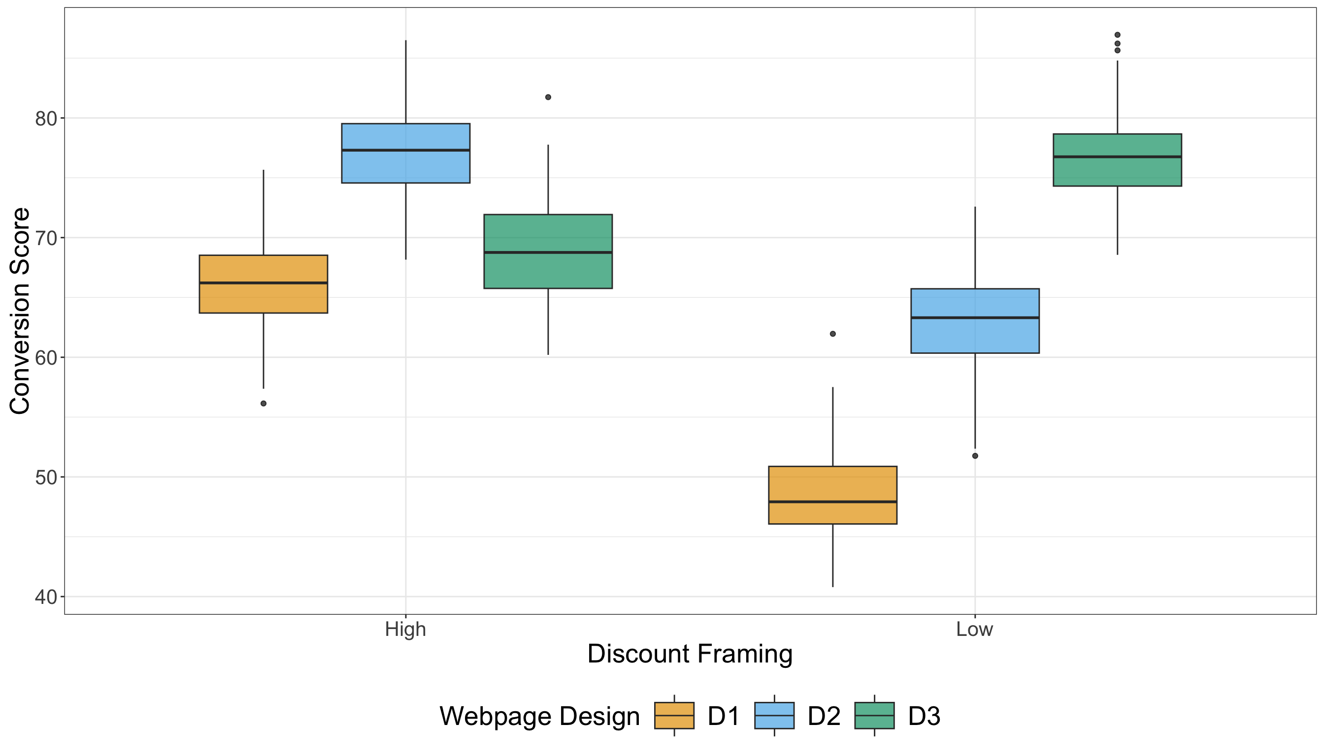
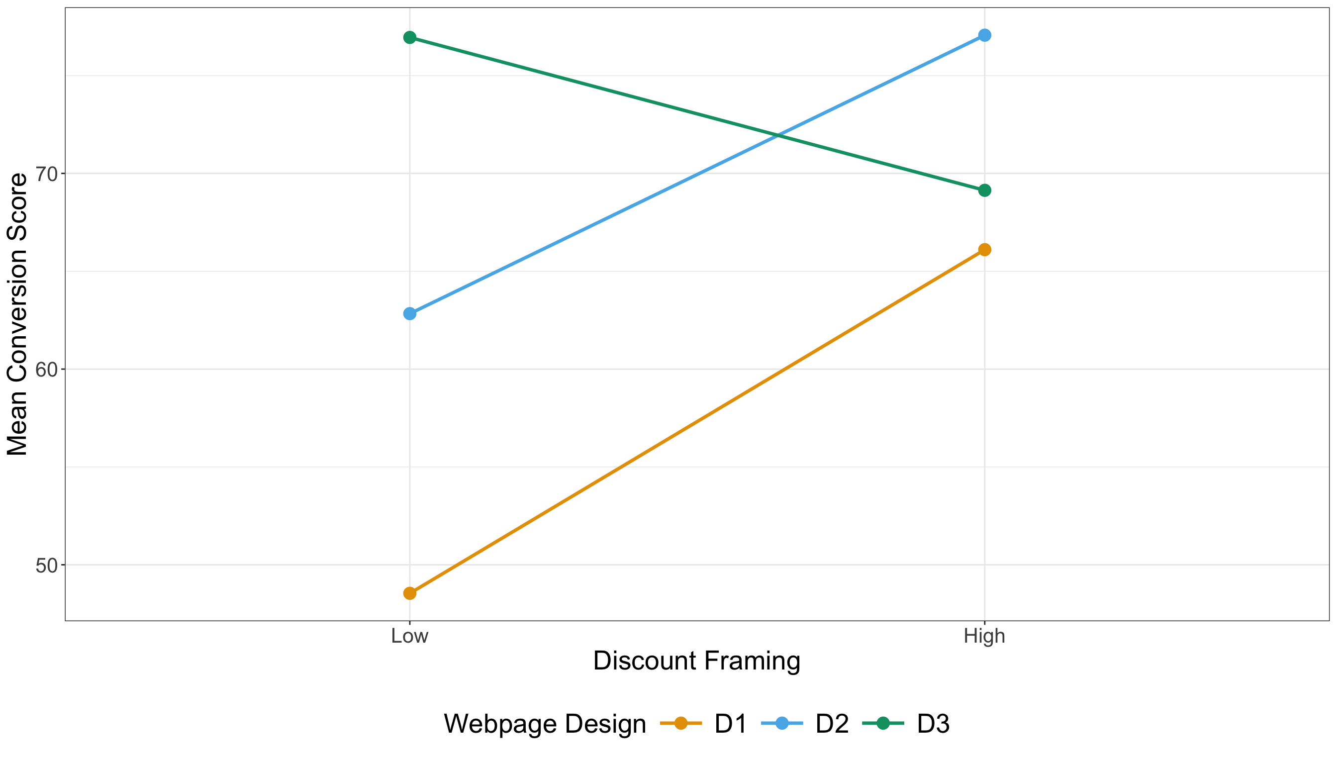
dtype: float644.2.3 Exploratory Data Analysis
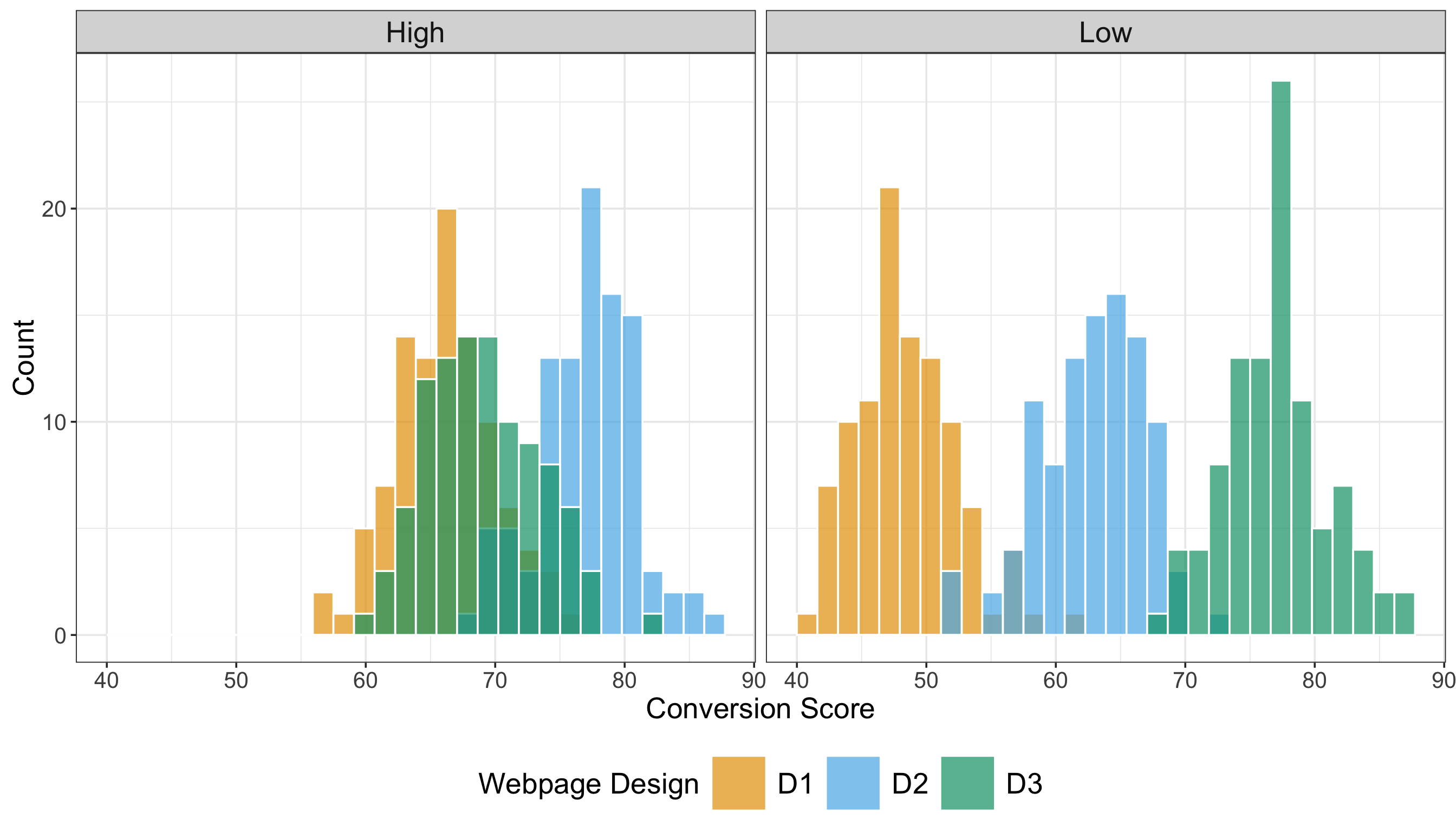
# Computing summaries
TwoWay_summary_table <- TwoWay_ABn_training |>
  group_by(checkout_design, discount_framing) |>
  summarise(
    mean_conversion = round(mean(conversion_score), 2),
    sd_conversion = round(sd(conversion_score), 2),
    n = n()
  ) |>
  arrange(checkout_design, discount_framing)
TwoWay_summary_table
# A tibble: 6 × 5
# Groups: checkout_design [3]
checkout_design discount_framing mean_conversion sd_conversion n
<chr> <chr> <dbl> <dbl> <int>
1 D1 High 66.1 3.79 100
2 D1 Low 48.5 3.89 100
3 D2 High 77.1 3.73 100
4 D2 Low 62.8 4.04 100
5 D3 High 69.1 4.27 100
6 D3 Low 77.0 3.91 100# Importing R training set via R library reticulate
TwoWay_ABn_training = r.TwoWay_ABn_training
# Computing summaries
TwoWay_summary_table = (
TwoWay_ABn_training
.groupby(["checkout_design", "discount_framing"])
.agg(
mean_conversion=("conversion_score", lambda x: round(np.mean(x), 2)),
sd_conversion=("conversion_score", lambda x: round(np.std(x, ddof=1), 2)),
n=("conversion_score", "count")
)
.reset_index()
.sort_values(["checkout_design", "discount_framing"])
)
TwoWay_summary_table| checkout_design | discount_framing | mean_conversion | sd_conversion | n | |
|---|---|---|---|---|---|
| 0 | D1 | High | 66.10 | 3.79 | 100 |
| 1 | D1 | Low | 48.54 | 3.89 | 100 |
| 2 | D2 | High | 77.07 | 3.73 | 100 |
| 3 | D2 | Low | 62.83 | 4.04 | 100 |
| 4 | D3 | High | 69.14 | 4.27 | 100 |
| 5 | D3 | Low | 76.95 | 3.91 | 100 |
4.2.4 Testing Settings
4.2.5 Hypothesis Definitions
4.2.6 Test Flavour and Components
# Running two-way ANOVA
TwoWay_aov <- aov(conversion_score ~ checkout_design * discount_framing,
  data = TwoWay_ABn_testing
)

# Displaying full two-way ANOVA table
TwoWay_aov <- tidy(TwoWay_aov) |>
  mutate(across(where(is.numeric) & !matches("p.value"), ~ round(.x, 2)))
TwoWay_aov
# A tibble: 4 × 6
term df sumsq meansq statistic p.value
<chr> <dbl> <dbl> <dbl> <dbl> <dbl>
1 checkout_design 2 26750. 13375. 817. 3.00e-171
2 discount_framing 1 8140. 8140. 497. 1.72e- 80
3 checkout_design:discount_framing 2 18207. 9103. 556. 7.93e-137
4 Residuals 594 9723. 16.4 NA NA # Importing R testing set via R library reticulate
TwoWay_ABn_testing = r.TwoWay_ABn_testing
# Running two-way ANOVA
TwoWay_model = ols('conversion_score ~ C(checkout_design) * C(discount_framing)', data=TwoWay_ABn_testing).fit()
TwoWay_aov = sm.stats.anova_lm(TwoWay_model, typ=2)
# Round all numeric columns except p-values
cols_to_round = [c for c in TwoWay_aov.columns if c != "PR(>F)"]
TwoWay_aov[cols_to_round] = TwoWay_aov[cols_to_round].round(2)
# Displaying full two-way ANOVA table
TwoWay_aov| sum_sq | df | F | PR(>F) | |
|---|---|---|---|---|
| C(checkout_design) | 26749.51 | 2.0 | 817.05 | 3.002041e-171 |
| C(discount_framing) | 8139.80 | 1.0 | 497.25 | 1.718558e-80 |
| C(checkout_design):C(discount_framing) | 18206.69 | 2.0 | 556.12 | 7.926552e-137 |
| Residual | 9723.46 | 594.0 | NaN | NaN |
4.2.7 Inferential Conclusions
# Extracting residuals
TwoWay_resid <- residuals(TwoWay_aov)

# Running Shapiro–Wilk test
TwoWay_shapiro <- shapiro.test(TwoWay_resid)

# Displaying outputs
tidy(TwoWay_shapiro) |>
  mutate_if(is.numeric, round, 2)
# A tibble: 1 × 3
statistic p.value method
<dbl> <dbl> <chr>
1 1 0.19 Shapiro-Wilk normality test# Extracting residuals
TwoWay_resid = TwoWay_model.resid
# Running Shapiro–Wilk tests
TwoWay_shapiro = shapiro(TwoWay_resid)
# Displaying outputs
TwoWay_shapiro = pd.DataFrame({
"W Statistic": [round(TwoWay_shapiro.statistic, 2)],
"p-value": [round(TwoWay_shapiro.pvalue, 2)]
})
TwoWay_shapiro| W Statistic | p-value | |
|---|---|---|
| 0 | 1.0 | 0.19 |
# Loading library
library(car)

# Running Levene test
TwoWay_levene <- leveneTest(conversion_score ~ as.factor(checkout_design) * as.factor(discount_framing),
  data = TwoWay_ABn_testing
)

# Displaying outputs
tidy(TwoWay_levene) |>
  mutate_if(is.numeric, round, 2)
# A tibble: 1 × 4
statistic p.value df df.residual
<dbl> <dbl> <dbl> <dbl>
1 1.92 0.09 5 594# Running Levene test
TwoWay_ABn_testing["group"] = TwoWay_ABn_testing["checkout_design"].astype(str) + "_" + TwoWay_ABn_testing["discount_framing"].astype(str)
groups_TwoWay = [group["conversion_score"].values for _, group in TwoWay_ABn_testing.groupby("group")]
stat1, p1 = levene(*groups_TwoWay)
# Displaying outputs
TwoWay_levene = pd.DataFrame({
"Levene Statistic": [round(stat1, 2)],
"p-value": [round(p1, 2)]
})
TwoWay_levene| Levene Statistic | p-value | |
|---|---|---|
| 0 | 1.92 | 0.09 |