5 Chi-squared Tests

The chi-square test is a non-parametric statistical test used for categorical data. Chi-square tests are used to make statistical inferences about categorical variables. Depending on the research question and the number of categorical variables, the specific chi-square test can differ, so it is important to identify the correct scenario for application.

The core idea behind chi-square tests is to compare observed counts with expected counts based on a population or theoretical distribution.

5.1 Hypotheses

Null hypothesis (\(H_0\)): The observed counts (\(O_i\)) and expected counts (\(E_i\)) are equal.
Alternative hypothesis (\(H_1\)): The observed counts (\(O_i\)) and expected counts (\(E_i\)) are not equal.

5.1.1 Test Statistic

The chi-square test statistic is calculated as:

\[ \chi^2 = \sum \frac{(O_i - E_i)^2}{E_i} \]

Under the null hypothesis, this statistic follows a chi-square distribution with degrees of freedom that depend on the type of test being performed.

Intuitively:
- If the observed and expected counts are close, the test statistic is small and not significant.
- If the observed counts differ substantially from the expected counts, the test statistic is large and significant, indicating a meaningful difference between the sample and the expected distribution.

5.1.2 Assumptions

Observations are independent.
Expected counts are sufficiently large (typically greater than 5).

The chi-square distribution is defined by its degrees of freedom, which vary depending on the test design and the number of categories.

There are two main types of chi-square tests:

Goodness-of-Fit Test
- Compares observed frequencies to expected frequencies for a single categorical variable.
- Example: Do the proportions of penguin species in the dataset match a hypothesized distribution (45% Adelie, 35% Gentoo, 20% Chinstrap)?
Test of Independence (or Homogeneity)
- Tests whether two categorical variables are independent.
- Example: Is penguin species independent of the island they were observed on?

5.2 (i) Chi-Square Goodness-of-Fit Test

This test examines whether the distribution of a categorical variable matches a hypothesized distribution.

5.2.1 Hypotheses

\(H_0\): The observed distribution matches the expected distribution.
\(H_1\): The observed distribution does not match the expected distribution.

5.2.2 Study Design

Suppose we hypothesize that the penguin species occur in the following proportions:

Adelie: 45%
Gentoo: 35%
Chinstrap: 20%

We want to test whether the observed species distribution in the Palmer Penguins dataset matches these proportions.

5.2.3 Data Collection & Wrangling

Here, we first load the Palmer Penguins dataset and remove any missing values to ensure complete observations. Next, we count how many penguins of each species are observed and calculate the expected counts based on our hypothesized proportions. These observed and expected frequencies will later be compared using the Chi-square test statistic.

R Code
Python Code

library(tidyverse)

── Attaching core tidyverse packages ──────────────────────── tidyverse 2.0.0 ──
✔ dplyr     1.1.4     ✔ readr     2.1.5
✔ forcats   1.0.1     ✔ stringr   1.5.2
✔ ggplot2   4.0.0     ✔ tibble    3.3.0
✔ lubridate 1.9.4     ✔ tidyr     1.3.1
✔ purrr     1.1.0     
── Conflicts ────────────────────────────────────────── tidyverse_conflicts() ──
✖ dplyr::filter() masks stats::filter()
✖ dplyr::lag()    masks stats::lag()
ℹ Use the conflicted package (<http://conflicted.r-lib.org/>) to force all conflicts to become errors

library(dplyr)
library(ggplot2)
library(palmerpenguins)


Attaching package: 'palmerpenguins'

The following objects are masked from 'package:datasets':

    penguins, penguins_raw

# Load dataset
penguins_clean <- penguins %>% 
  drop_na()

# Count observed species
observed_counts <- table(penguins_clean$species)
print("Observed counts:")

[1] "Observed counts:"

print(observed_counts)


   Adelie Chinstrap    Gentoo 
      146        68       119

# Expected proportions
expected_props <- c(0.45, 0.35, 0.20)

# Convert to expected counts
n <- nrow(penguins_clean)
expected_counts <- expected_props * n
print("Expected counts (based on proportions):")

[1] "Expected counts (based on proportions):"

print(expected_counts)

[1] 149.85 116.55  66.60

import seaborn as sns
import pandas as pd

# Load dataset
penguins = sns.load_dataset("penguins")

# Drop rows with missing values
penguins_clean = penguins.dropna()

# Count observed species
observed_counts = penguins_clean["species"].value_counts()
print("Observed counts:")

Observed counts:

print(observed_counts)

species
Adelie       146
Gentoo       119
Chinstrap     68
Name: count, dtype: int64

# Expected proportions
expected_props = [0.45, 0.35, 0.20]

# Convert to expected counts
n = len(penguins_clean)
expected_counts = [p * n for p in expected_props]

print("\nExpected counts (based on proportions):")


Expected counts (based on proportions):

print(expected_counts)

[149.85, 116.55, 66.60000000000001]

5.2.4 Exploratory Data Analysis (EDA)

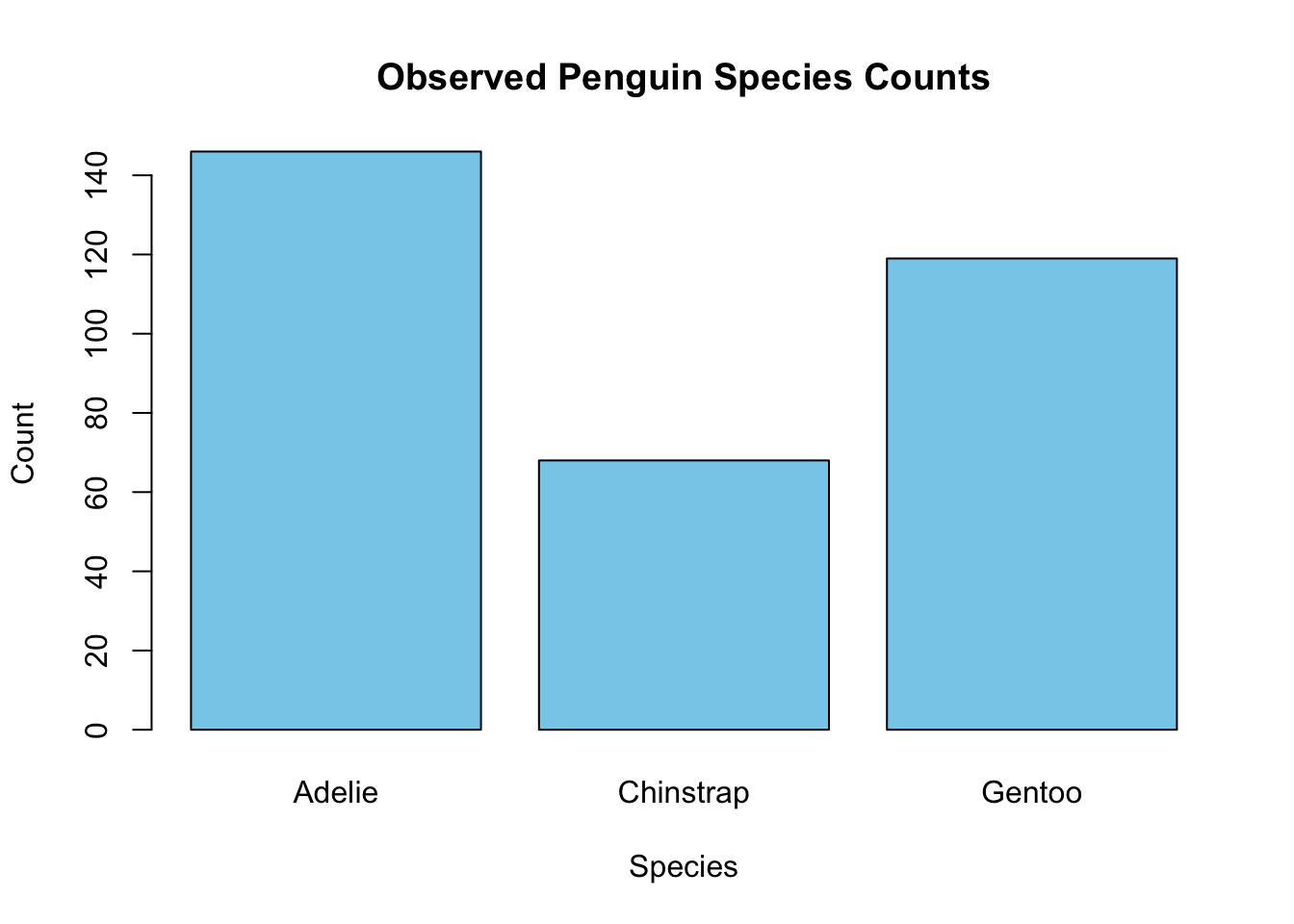
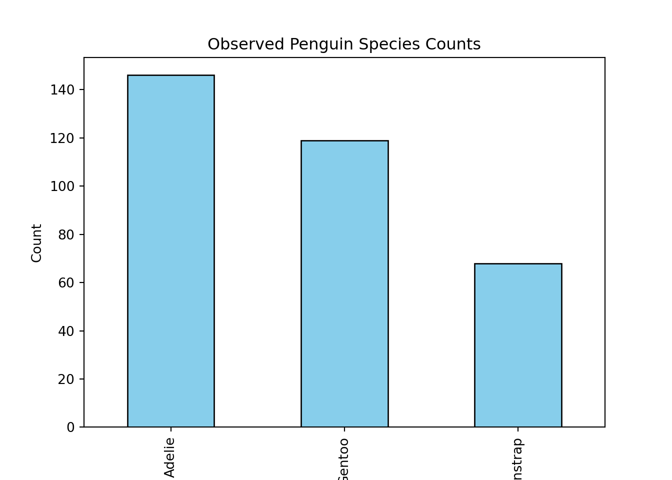
Before running the statistical test, it’s helpful to visualize the observed counts. A simple bar plot allows us to see whether any species appear more or less frequent than expected, which helps build intuition about potential differences.

R Code
Python Code

# Bar plot of observed counts
barplot(
  observed_counts,
  col = "skyblue",
  border = "black",
  main = "Observed Penguin Species Counts",
  xlab = "Species",
  ylab = "Count"
)

import matplotlib.pyplot as plt

observed_counts.plot(kind="bar", color="skyblue", edgecolor="black")
plt.title("Observed Penguin Species Counts")
plt.xlabel("Species")
plt.ylabel("Count")
plt.show()

5.2.5 Implementation

Now we apply the Chi-square goodness-of-fit test, comparing observed and expected counts. The test statistic measures how far the observed frequencies deviate from the expected ones. A large value suggests that the observed distribution differs significantly from what was hypothesized.

R Code
Python Code

# Chi-square goodness-of-fit test
chi2_test <- chisq.test(
  x = observed_counts,
  p = expected_props
)
print(chi2_test)


    Chi-squared test for given probabilities

data:  observed_counts
X-squared = 61.551, df = 2, p-value = 4.31e-14

from scipy.stats import chisquare

chi2_stat, p_value = chisquare(
    f_obs=observed_counts,
    f_exp=expected_counts
)
print(f"Chi-square = {chi2_stat:.3f}, p = {p_value:.4f}")

Chi-square = 0.180, p = 0.9140

5.2.6 Interpretation

If \(p < 0.05\): Reject \(H_0\) → the species distribution differs significantly from the expected proportions.

If \(p \ge 0.05\): Fail to reject \(H_0\) → no significant difference.

5.3 (ii) Chi-Square Test of Independence

This test evaluates whether two categorical variables are independent.

5.3.1 Hypotheses

\(H_0\): The two categorical variables are independent.

\(H_1\): The two categorical variables are not independent (they are associated).

5.3.2 Study Design

We want to test whether penguin species is independent of island — in other words, whether certain species are more common on certain islands.

5.3.3 Data Collection & Wrangling

We create a contingency table summarizing the counts of species across islands. This table serves as the basis for calculating expected frequencies and testing independence.

R Code
Python Code

# Contingency table: species vs island
contingency_table <- table(
  penguins_clean$species,
  penguins_clean$island
)
print("Contingency table:")

[1] "Contingency table:"

print(contingency_table)

           
            Biscoe Dream Torgersen
  Adelie        44    55        47
  Chinstrap      0    68         0
  Gentoo       119     0         0

# Create contingency table: species vs island
contingency_table = pd.crosstab(
    penguins_clean["species"], 
    penguins_clean["island"]
)
print("Contingency table:")

Contingency table:

print(contingency_table)

island     Biscoe  Dream  Torgersen
species                            
Adelie         44     55         47
Chinstrap       0     68          0
Gentoo        119      0          0

5.3.4 Exploratory Data Analysis (EDA)

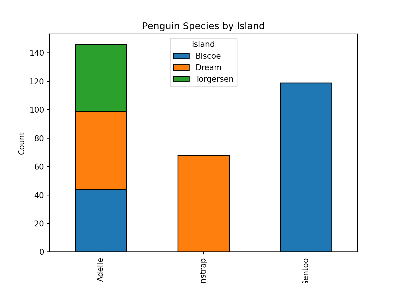
Visualizing the contingency table helps us see any apparent association between species and island. If bars differ noticeably in height across islands, it hints that species distribution might depend on island location.

R Code
Python Code

# Stacked bar plot of species by island
barplot(
  contingency_table,
  col = c("orange", "skyblue", "green"),
  border = "black",
  main = "Penguin Species by Island",
  xlab = "Species",
  ylab = "Count",
  legend.text = TRUE
)

contingency_table.plot(
    kind="bar", stacked=True, edgecolor="black"
)
plt.title("Penguin Species by Island")
plt.xlabel("Species")
plt.ylabel("Count")
plt.show()

5.3.5 Implementation

We now apply the Chi-square test of independence to evaluate whether the distribution of species differs by island. If the test is significant, it suggests a relationship between the two categorical variables.

R Code
Python Code

# Chi-square test of independence
chi2_indep <- chisq.test(contingency_table)
print(chi2_indep)


    Pearson's Chi-squared test

data:  contingency_table
X-squared = 284.59, df = 4, p-value < 2.2e-16

from scipy.stats import chi2_contingency

chi2_stat, p_value, dof, expected = chi2_contingency(contingency_table)

print(f"Chi-square = {chi2_stat:.3f}, df = {dof}, p = {p_value:.4f}")

Chi-square = 284.590, df = 4, p = 0.0000

5.3.6 Interpretation

If \(p < 0.05\): Reject \(H_0\) → species and island are not independent (association exists).

If \(p \ge 0.05\): Fail to reject \(H_0\) → species and island appear independent.